Selecting a mobility model • nomad

Once we have prepared a set of regions for an analysis, we still need to decide which mobility model to use. Several models may be available for a country, and a model that fit its original data well may behave quite differently when applied to new populations and distances. This vignette works through those choices using the Zambia Facebook models, from inspecting their source data to comparing predictions and combining them in an ensemble.

All the examples use data included with nomad, so you can follow them without access to the private trip matrices used for fitting. Longer setup and plotting blocks are folded below their descriptions. Prediction warnings are also kept in expandable panels beside the relevant result, where you can read how our example differs from the fitted setting.

library(nomad)

Find a relevant source

Let’s start by looking at the datasets available for Zambia. Finding data from the country of interest is useful, but we also need to consider whose movement was recorded and at what spatial scale. For example, journeys between large administrative areas may have a different relationship with distance from journeys between small urban neighbourhoods. The source metadata help us identify these differences before we compare the fitted models.

The table below includes whether each dataset has fitted models available. Entries with has_fitted_models = FALSE describe data in the catalogue for which we do not yet have models to use for prediction.

mobility_table(country = "ZMB")[, c(
  "name", "aggregation", "has_fitted_models", "prediction_period_days", "distance_unit"
)]

#> # A tibble: 3 × 5
#>   name        aggregation has_fitted_models prediction_period_days distance_unit
#>   <chr>       <chr>       <lgl>                              <dbl> <chr>        
#> 1 zmb_cdr_20… admin_2     TRUE                                  NA m            
#> 2 zmb_fb_2020 admin_2     TRUE                                  NA km           
#> 3 zmb_fb_2025 admin_2     TRUE                                  21 m

We will use zmb_fb_2025 for the comparison below. Its predictions represent trip counts over 21 days. This period is separate from the start and end dates over which the observations were collected. Averaging a series of matrices retains the 21-day period represented by each matrix, rather than making the counts refer to the whole collection window.

Datasets and models can be shared through nomad even when some of their source metadata are unavailable. For example, the earlier Zambia Facebook and CDR models from 2020 do not include a prediction period. Their predicted patterns of movement can still be explored, but we cannot interpret the counts as trips per day or convert them to a chosen duration. Looking at metadata completeness therefore helps us decide which models can support the analysis we have in mind.

Compare fits to the same observations

Several model families were fit to these observations. We can retrieve them with model_table() and compare their root mean squared error (RMSE), which summarises the differences between fitted and observed flows. A lower RMSE means that the model reproduced these particular observations more closely. This is a useful first comparison, although it does not establish how well that model will predict movement elsewhere. The table also tells us whether each family supports prediction for new regions, which we will need later in the example.

candidates <- model_table(data_name = "zmb_fb_2025")
knitr::kable(candidates[, c("model_type", "mobility_model", "RMSE", "max_rhat", "supports_newdata")],
             digits = 2, col.names = c("Type", "Family", "RMSE", "Maximum R-hat", "New regions"))

Type	Family	RMSE	Maximum R-hat	New regions
exp	departure-diffusion	946017.6	1.01	TRUE
power	departure-diffusion	946520.7	1.01	TRUE
radiation	departure-diffusion	946972.8	1.01	TRUE
basic	gravity	819787889.5	1.00	TRUE
exp	gravity	947086.4	1.05	TRUE
exp_norm	gravity	965441.9	1.01	TRUE
power	gravity	942100.3	1.55	TRUE
power_norm	gravity	946881.4	1.00	TRUE
scaled_power	gravity	952655.1	1.03	TRUE
transport	gravity	1057907.1	1.00	TRUE
basic	radiation	831655.6	NA	FALSE
finite	radiation	833481.7	NA	FALSE

Before choosing the model with the smallest error, it is also useful to look at max_rhat. R-hat compares variation within and between the chains used to fit the model. A high value raises a concern that the chains have not converged, so the reported parameter estimates need further review even if the fit error is small. The package preserves the supplied fits and flags values above 1.1 through rhat_above_1_1. You can inspect individual parameters with summary(model); being below the flag threshold does not by itself establish that a fit is reliable.

We can use the available RMSE values to calculate a set of model weights. The chosen statistic needs to be available for every model in the comparison. For example, the deviance information criterion (DIC) was not calculated for these fits, so we cannot use it to derive their weights.

These fit-based weights are most interpretable when the models were fit to the same observations. Across different datasets, differences in trip counts, spatial aggregation and sampling can change the scale of the errors. Combining those errors would then mix differences in the data with differences in model performance. For this reason, model_weights() requires the models to share a source dataset. If we want to compare models from different sources, we can choose manual weights and examine how our results change across those choices, making clear that the weights describe a sensitivity analysis.

weights <- model_weights(data_name = "zmb_fb_2025", metric = "RMSE")
knitr::kable(weights[, c("name", "RMSE", "weight")], digits = c(0, 1, 3))

name	RMSE	weight
zmb_fb_2025_mod_dd_exp	946017.6	0.090
zmb_fb_2025_mod_dd_power	946520.7	0.090
zmb_fb_2025_mod_dd_radiation	946972.8	0.090
zmb_fb_2025_mod_grav_basic	819787889.5	0.000
zmb_fb_2025_mod_grav_exp	947086.4	0.090
zmb_fb_2025_mod_grav_exp_norm	965441.9	0.088
zmb_fb_2025_mod_grav_power	942100.3	0.090
zmb_fb_2025_mod_grav_power_norm	946881.4	0.090
zmb_fb_2025_mod_grav_scaled_power	952655.1	0.089
zmb_fb_2025_mod_grav_transport	1057907.1	0.080
zmb_fb_2025_mod_rad_basic	831655.6	0.102
zmb_fb_2025_mod_rad_finite	833481.7	0.102

For these fits, the RMSE weights are proportional to the inverse error and normalised to sum to one. A model with half the error of another therefore receives twice its weight. This summarises relative fit to the Zambia observations, but does not tell us how similar our prediction setting is to the source setting or give a probability that each model is correct. We will therefore inspect the models and their predictions before deciding how to combine them.

Inspect the source and diagnostics

For the rest of this example we will compare normalised exponential gravity with exponential departure-diffusion, both fit to zmb_fb_2025. Each has a stored maximum R-hat of 1.01 and minimum effective sample sizes above 600. The effective sample size accounts for similarity between successive draws, so it can be much smaller than the number of samples stored. These summaries help us choose examples with more reassuring sampling diagnostics, although a full convergence assessment would also require inspecting the chains themselves.

We can use model_profile() to see the distance units, population scale and prediction period associated with a model. The saved fit checks then let us compare its predictions with the original observations, even though the private trip matrix itself is not distributed with the package.

gravity <- model_db$zmb_fb_2025_mod_grav_exp_norm
departure <- model_db$zmb_fb_2025_mod_dd_exp
model_profile(gravity)

#> # A tibble: 1 × 27
#>   name  data_name country aggregation date_start date_end   source_duration_days
#>   <chr> <chr>     <chr>   <chr>       <date>     <date>                    <dbl>
#> 1 zmb_… zmb_fb_2… ZMB     admin_2     2024-07-29 2025-06-16                   21
#> # ℹ 20 more variables: prediction_period_days <dbl>, distance_unit <chr>,
#> #   supports_newdata <lgl>, supports_stochastic_draws <lgl>, n_origin <int>,
#> #   n_dest <int>, distance_min <dbl>, distance_q25 <dbl>,
#> #   distance_median <dbl>, distance_q75 <dbl>, distance_max <dbl>,
#> #   population_total <dbl>, population_min <dbl>, population_median <dbl>,
#> #   population_max <dbl>, max_rhat <dbl>, min_n_eff <dbl>,
#> #   rhat_above_1_1 <lgl>, has_mobility_data <lgl>, has_saved_check <lgl>

check(gravity, plots = FALSE)

#> $DIC
#> [1] NA
#> 
#> $RMSE
#> [1] 965441.9
#> 
#> $MAPE
#> [1] 32.18002
#> 
#> $R2
#> [1] 0.1056686

plot(gravity)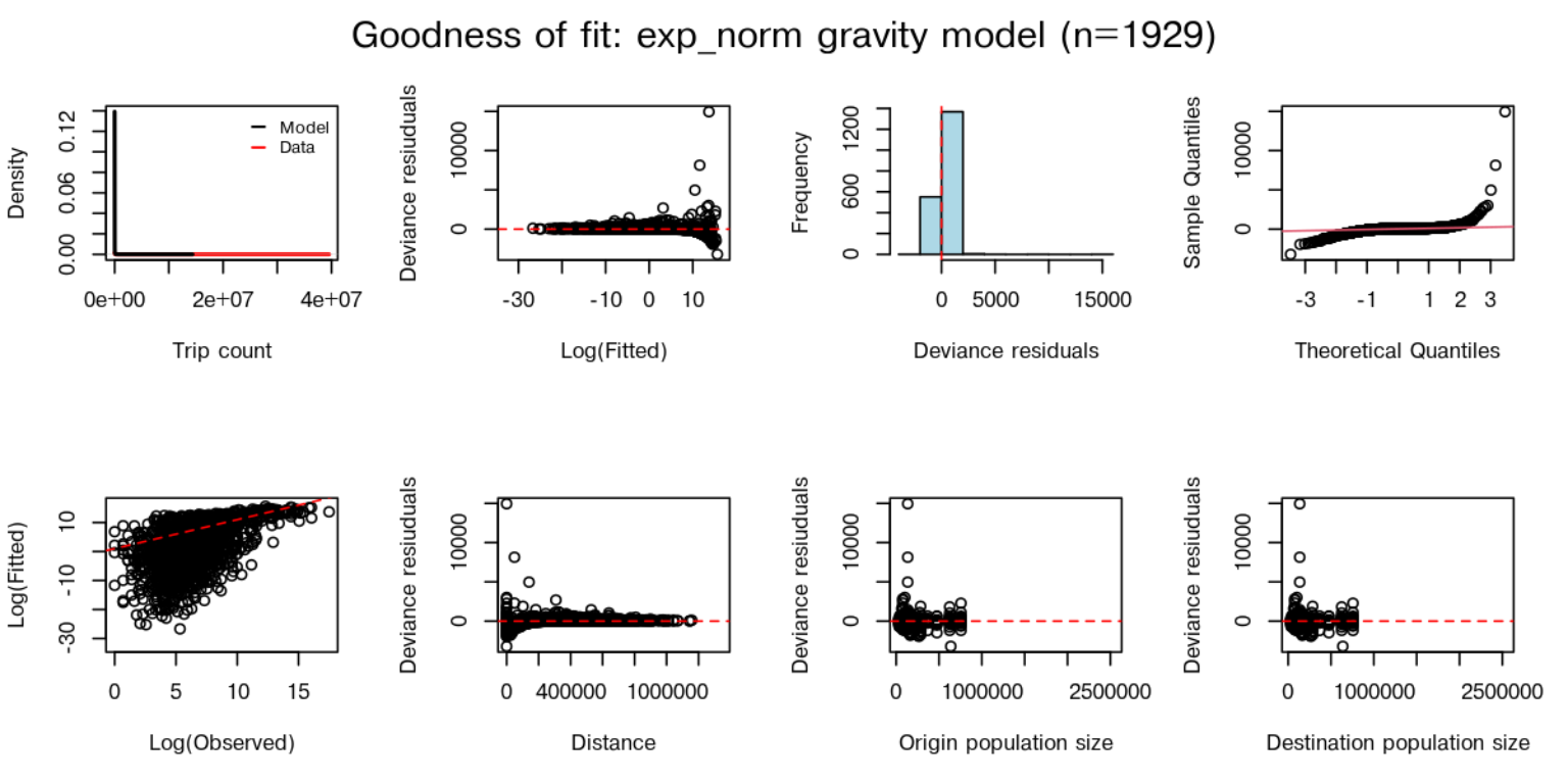

Observed and fitted flows for Zambia exponential gravity

In the observed-versus-predicted panel, flows near the line of agreement are those the model reproduces closely. Look for groups of flows that are consistently overpredicted or underpredicted, and for patterns in the residual panel. For example, a model might fit the largest flows reasonably well while missing many small ones, which could matter when studying movement into less connected areas.

These checks describe the source fit. Before using it for our own regions, we also need to check whether their distances and populations are comparable, and whether the model can accept the inputs we want to provide. The next step sets up a small prediction request so we can work through those checks.

Prepare a common prediction setting

To keep the matrices small enough to inspect, we will use eight regions from the distances and populations used for fitting. The distance matrix D has origins in its rows and destinations in its columns, while N gives the population of each region. We keep the region names on both inputs so that nomad can match the populations to the correct rows and columns. For your own analysis, these would be the distances and population estimates prepared for your study regions.

source <- gravity$get_model()$data
regions <- rownames(source$D)[1:8]
newdata <- list(
  D = source$D[regions, regions],
  N = source$N_orig[regions]
)

The source distances are measured in metres, so we supply unit = "m" when predicting. This tells nomad how to interpret our input distances. It can then convert them to the units used by each fitted model, which is particularly useful when comparing models whose original data used different units.

Although we have kept the source populations for these eight regions, we have removed the remaining regions from the prediction setting. The warnings about fewer regions and a smaller total population draw attention to this change. For a model that distributes movement across the available destinations, removing destinations can change the remaining flows. These predictions therefore describe a new, smaller setting; they should not be treated as simply extracting eight rows and columns from a prediction for the full source population.

a <- predict(gravity, newdata = newdata, unit = "m", duration = 21)

b <- predict(departure, newdata = newdata, unit = "m", duration = 21)

round(a[1:4, 1:4])

#>            destination
#> origin      ZMB.1.1_1 ZMB.1.2_1 ZMB.1.3_1 ZMB.1.4_1
#>   ZMB.1.1_1   5822213    268155        15      3706
#>   ZMB.1.2_1     60209   1307265        31        57
#>   ZMB.1.3_1         3        27   1101759         0
#>   ZMB.1.4_1       995        68         0   1562487

Show prediction warnings

#> Warning: ! Prediction data have far fewer regions than the fitted source data.
#> ℹ `newdata` has "8" regions; the fitted model has "115".
#> • Predictions may be coarser than the source data can support.

#> Warning: ! Prediction population is much smaller than the fitted source population.
#> ℹ `newdata` population: "1538603"; fitted model source population: "18296043".
#> • Check that this model is suitable for the population scale being predicted.

#> Warning: ! Prediction data have far fewer regions than the fitted source data.
#> ℹ `newdata` has "8" regions; the fitted model has "115".
#> • Predictions may be coarser than the source data can support.
#> ! Prediction population is much smaller than the fitted source population.
#> ℹ `newdata` population: "1538603"; fitted model source population: "18296043".
#> • Check that this model is suitable for the population scale being predicted.

Each entry is a predicted trip count from its row region to its column region over 21 days. The counts can include repeated trips by the same person. If we requested 42 days, the package would double these values, assuming the same average daily trip rate throughout. That conversion cannot describe seasonal changes or changes in travel behaviour.

This conversion depends on having a source prediction period. For models shared without that information, leaving duration unset returns the unscaled prediction with a warning. Requesting a conversion instead raises an error, since the package cannot calculate the multiplier. Such a model may still help us explore relative movement, but we would need the missing metadata before using its predictions as trip counts over a specified period.

Recognise unsupported requests

Basic and finite radiation models retain predictions for their exact original regions and populations. They cannot transfer the stored matrix to the eight-region subset above. nomad rejects that request directly, including through an ensemble, and explains how to choose a model that supports new regions or recalculate radiation with mobility when you have the necessary trip totals. For the original regions, we can retrieve the stored prediction without supplying new inputs, as below.

radiation <- model_db$zmb_fb_2025_mod_rad_basic
original <- predict(radiation)
dim(original)

#> [1] 115 115

For model families that support new inputs, a different country, spatial scale or population may still be a valid prediction request. The warnings identify those differences so that we can consider whether transferring the fitted parameters is reasonable. Country checks require locations, supplied as an sf object or a longitude/latitude table, because distances alone do not locate the regions geographically. None of the bundled models was fit to international travel, so a prediction between countries would require assumptions beyond what those source data can establish.

Inspect uncertainty

The predictions above use the mean estimates of the fitted parameters. To explore how the stored parameter uncertainty affects the predicted flows, we can request 100 simulations with nsim = 100. For a model that supports these simulations, the result is an array containing one mobility matrix per draw. We can then use uncertainty_summary() to look at quantities such as the total number of trips and the number travelling between different regions.

The current mobility predictor samples each parameter independently from a normal distribution truncated at zero, using its stored mean and standard deviation. The draws therefore approximate the uncertainty in each parameter separately. They do not preserve relationships between parameters in the original Markov chain Monte Carlo (MCMC) samples. These predictions also leave out observation noise, uncertainty in populations or distances, and uncertainty about applying the model in another setting.

draws <- predict(gravity, newdata = newdata, unit = "m", nsim = 100, seed = 42)

uncertainty_summary(draws, metrics = c("total", "between_region", "max"))

#> # A tibble: 9 × 3
#>   metric          prob     value
#>   <chr>          <dbl>     <dbl>
#> 1 total          0.025 21374078.
#> 2 total          0.5   21377435.
#> 3 total          0.975 21380787.
#> 4 between_region 0.025  3760995.
#> 5 between_region 0.5    3762604.
#> 6 between_region 0.975  3763534.
#> 7 max            0.025  5821286.
#> 8 max            0.5    5822177.
#> 9 max            0.975  5823186.

selected <- uncertainty_matrices(draws, metric = "between_region", probs = c(0.1, 0.5, 0.9))
attr(selected, "selected")

#> # A tibble: 3 × 4
#>   name   prob simulation    value
#>   <chr> <dbl>      <int>    <dbl>
#> 1 q0.1    0.1         71 3761533.
#> 2 q0.5    0.5         46 3762591.
#> 3 q0.9    0.9         54 3763218.

Show prediction warnings

#> Warning: ! Prediction data have far fewer regions than the fitted source data.
#> ℹ `newdata` has "8" regions; the fitted model has "115".
#> • Predictions may be coarser than the source data can support.

#> Warning: ! Prediction population is much smaller than the fitted source population.
#> ℹ `newdata` population: "1538603"; fitted model source population: "18296043".
#> • Check that this model is suitable for the population scale being predicted.

To visualise the variation, we select draws near the 10th, 50th and 90th percentiles of between-region movement. Each selected matrix comes from one complete draw, preserving the pattern of flows that its parameters produced. Taking a separate quantile in every cell could instead assemble a matrix that was never predicted by any one parameter draw. If we ranked by a different quantity, such as the largest individual flow, we might select different matrices.

The three heatmaps use a common colour scale so that a given colour means the same number of trips in each panel. The scale uses log(1 + trips), allowing both large and small flows, including zeros, to remain visible.

plot_uncertainty(draws, metric = "between_region", probs = c(0.1, 0.5, 0.9))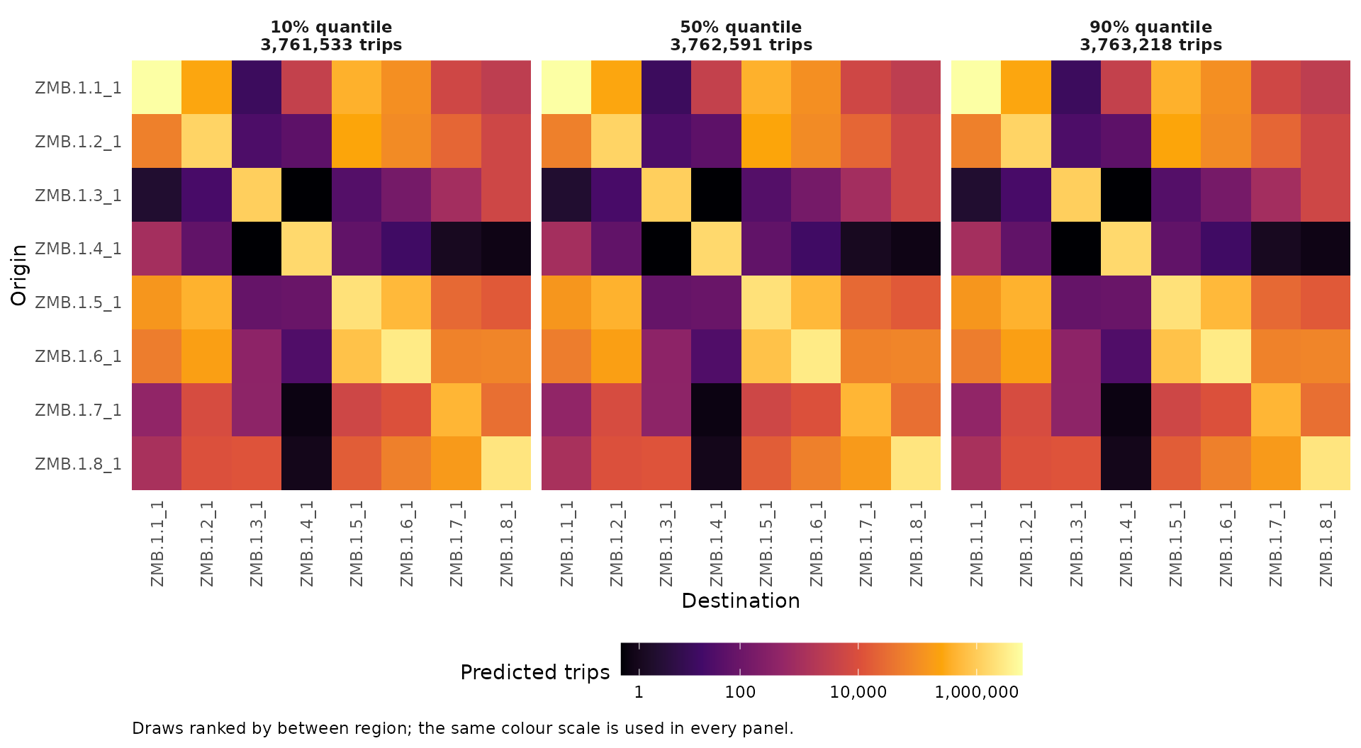

Lower, median and upper mobility matrices selected by between-region movement

The small difference between these panels is present in the supplied fit. We can check its parameter summaries and quantify the spread in between-region trips:

parameter_summary <- gravity$get_model()$summary[, c("mean", "sd")]
parameter_summary

#>               mean           sd
#> delta 2.897039e+04 2.454642e+00
#> omega 3.129614e-07 3.045025e-07
#> theta 1.389407e+01 1.247901e-03

between <- mobility_metrics(draws)$between_region
interval <- stats::quantile(between, c(0.1, 0.5, 0.9))
relative_width <- 100 * (interval[3] - interval[1]) / interval[2]

For these 100 draws, the 10th-to-90th percentile interval is only 0.045% of the median between-region trip total. The movement-rate parameter theta and distance parameter delta have very small stored standard deviations relative to their means. In this normalised gravity model, total trips are theta * sum(N), which also constrains variation in the total. The destination-population exponent omega is close to zero, so destination population contributes little to differences between flows in this fit.

The narrow spread therefore reflects the stored parameter summaries and the prediction method for this particular fitted model. It would be misleading to interpret it as the full uncertainty about travel in these regions, since it omits the other sources described above. Increasing nsim would estimate the same approximate distribution more precisely, but would not account for those missing sources. To investigate uncertainty about model choice, we can instead compare the predictions from different plausible models, as in the next section.

Compare and combine predictions

We now have two predictions for the same target regions and period, so we can compare their entries directly. Using gravity as the baseline, a positive value from prediction_difference(b, a) means that departure-diffusion predicts more trips for that origin-destination pair. The function matches region names if their order differs, and raises an error if the matrices refer to different sets of target regions.

We can also combine the two models in an ensemble. The example below gives 60% of the weight to gravity and 40% to departure-diffusion, then compares the total predicted trips with those from each component.

round(prediction_difference(b, a)[1:4, 1:4])

#>            destination
#> origin      ZMB.1.1_1 ZMB.1.2_1 ZMB.1.3_1 ZMB.1.4_1
#>   ZMB.1.1_1  -1128508    307408     15413    114280
#>   ZMB.1.2_1     44364    -67050      6347      7896
#>   ZMB.1.3_1      9617     21863   -314477       634
#>   ZMB.1.4_1    225565     83989      1951   -452055

ensemble <- nomad_ensemble(list(gravity = gravity, departure = departure),
                           weights = c(gravity = 0.6, departure = 0.4))
combined <- predict(ensemble, newdata = newdata, unit = "m", duration = 21)

c(gravity = sum(a), departure = sum(b), ensemble = sum(combined))

#>   gravity departure  ensemble 
#>  21377461  21763957  21532059

Show prediction warnings

#> Warning: ! Prediction data have far fewer regions than the fitted source data.
#> ℹ `newdata` has "8" regions; the fitted model has "115".
#> • Predictions may be coarser than the source data can support.

#> Warning: ! Prediction population is much smaller than the fitted source population.
#> ℹ `newdata` population: "1538603"; fitted model source population: "18296043".
#> • Check that this model is suitable for the population scale being predicted.

#> Warning: ! Prediction data have far fewer regions than the fitted source data.
#> ℹ `newdata` has "8" regions; the fitted model has "115".
#> • Predictions may be coarser than the source data can support.

#> Warning: ! Prediction population is much smaller than the fitted source population.
#> ℹ `newdata` population: "1538603"; fitted model source population: "18296043".
#> • Check that this model is suitable for the population scale being predicted.

Here the weights are choices we have made for the example. We could give the models equal influence or calculate fit-based weights for these two models, provided we are satisfied that their fit statistics are an appropriate basis for the comparison. The weights calculated earlier included every model for the dataset, so we would need to restrict that calculation to the components we intend to combine.

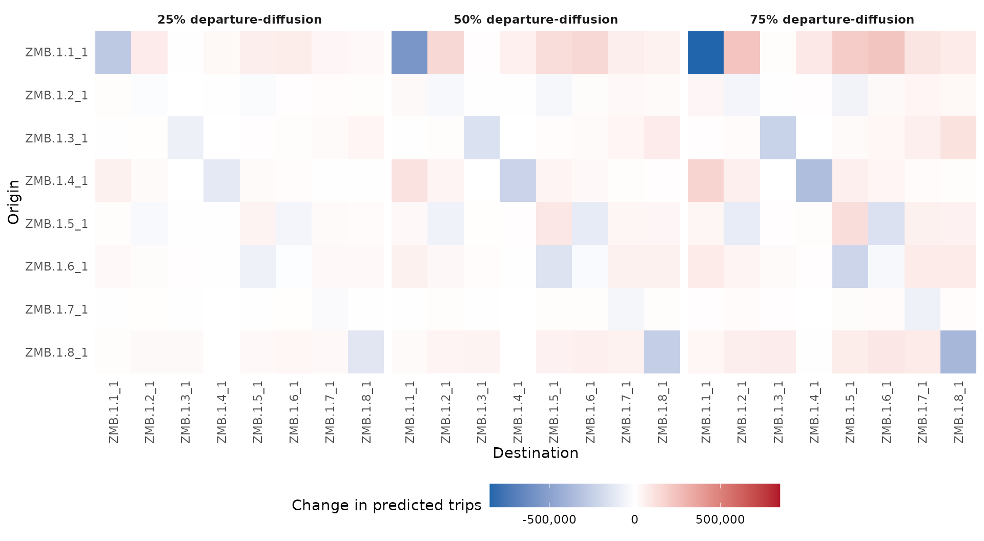
To see how those choices affect individual flows, compare three fixed weights against the gravity prediction. Each panel below shows ensemble minus gravity: red cells mean more trips than gravity predicts, blue cells mean fewer, and white means no change. Rows are origins and columns are destinations, including trips that stay within the same region on the diagonal.

All panels use the same colour limits, centred on zero. The weights are illustrative sensitivity choices, not estimates of which model is correct. With two fixed component matrices, the difference is weight * (departure - gravity), so the pattern stays the same while its magnitude changes. Here weight is the share given to departure-diffusion.

Show how to compare fixed ensemble weights

weights <- c(0.25, 0.5, 0.75)
differences <- lapply(weights, function(weight) {
  candidate <- nomad_ensemble(list(gravity = gravity, departure = departure),
                              weights = c(gravity = 1 - weight, departure = weight))
  prediction <- predict(candidate, newdata = newdata, unit = "m", duration = 21)
  cells <- as.data.frame(as.table(prediction_difference(prediction, a)))
  names(cells) <- c("origin", "destination", "difference")
  cells$weight <- paste0(100 * weight, "% departure-diffusion")
  cells
})
changes <- do.call(rbind, differences)
changes$origin <- factor(changes$origin, levels = rev(rownames(a)))
changes$destination <- factor(changes$destination, levels = colnames(a))
limit <- max(abs(changes$difference))

ggplot2::ggplot(changes, ggplot2::aes(destination, origin, fill = difference)) +
  ggplot2::geom_tile() +
  ggplot2::facet_wrap(~weight, nrow = 1) +
  ggplot2::scale_fill_gradient2(
    low = "#2166ac", mid = "white", high = "#b2182b",
    midpoint = 0, limits = c(-limit, limit),
    labels = function(x) format(x, big.mark = ",", scientific = FALSE, trim = TRUE)
  ) +
  ggplot2::scale_x_discrete(expand = c(0, 0)) +
  ggplot2::scale_y_discrete(expand = c(0, 0)) +
  ggplot2::labs(x = "Destination", y = "Origin", fill = "Change in predicted trips") +
  ggplot2::theme_minimal(base_size = 11) +
  ggplot2::theme(
    panel.grid = ggplot2::element_blank(),
    axis.text.x = ggplot2::element_text(angle = 90, hjust = 1, vjust = 0.5),
    strip.text = ggplot2::element_text(face = "bold"),
    legend.position = "bottom",
    legend.key.width = grid::unit(1.5, "cm")
  )

Difference from gravity predictions at 25, 50 and 75 percent departure-diffusion weight; red means more trips and blue means fewer, with one shared colour scale

Show prediction warnings

#> Warning: ! Prediction data have far fewer regions than the fitted source data.
#> ℹ `newdata` has "8" regions; the fitted model has "115".
#> • Predictions may be coarser than the source data can support.

#> Warning: ! Prediction population is much smaller than the fitted source population.
#> ℹ `newdata` population: "1538603"; fitted model source population: "18296043".
#> • Check that this model is suitable for the population scale being predicted.

#> Warning: ! Prediction data have far fewer regions than the fitted source data.
#> ℹ `newdata` has "8" regions; the fitted model has "115".
#> • Predictions may be coarser than the source data can support.

#> Warning: ! Prediction population is much smaller than the fitted source population.
#> ℹ `newdata` population: "1538603"; fitted model source population: "18296043".
#> • Check that this model is suitable for the population scale being predicted.

#> Warning: ! Prediction data have far fewer regions than the fitted source data.
#> ℹ `newdata` has "8" regions; the fitted model has "115".
#> • Predictions may be coarser than the source data can support.

#> Warning: ! Prediction population is much smaller than the fitted source population.
#> ℹ `newdata` population: "1538603"; fitted model source population: "18296043".
#> • Check that this model is suitable for the population scale being predicted.

#> Warning: ! Prediction data have far fewer regions than the fitted source data.
#> ℹ `newdata` has "8" regions; the fitted model has "115".
#> • Predictions may be coarser than the source data can support.

#> Warning: ! Prediction population is much smaller than the fitted source population.
#> ℹ `newdata` population: "1538603"; fitted model source population: "18296043".
#> • Check that this model is suitable for the population scale being predicted.

#> Warning: ! Prediction data have far fewer regions than the fitted source data.
#> ℹ `newdata` has "8" regions; the fitted model has "115".
#> • Predictions may be coarser than the source data can support.

#> Warning: ! Prediction population is much smaller than the fitted source population.
#> ℹ `newdata` population: "1538603"; fitted model source population: "18296043".
#> • Check that this model is suitable for the population scale being predicted.

#> Warning: ! Prediction data have far fewer regions than the fitted source data.
#> ℹ `newdata` has "8" regions; the fitted model has "115".
#> • Predictions may be coarser than the source data can support.

#> Warning: ! Prediction population is much smaller than the fitted source population.
#> ℹ `newdata` population: "1538603"; fitted model source population: "18296043".
#> • Check that this model is suitable for the population scale being predicted.

The heatmaps show which flows are most affected by changing the ensemble weights. Whether those differences matter will depend on what we use the mobility matrix for. For example, a modest difference in travel to a less connected region might change when an outbreak reaches it, even if the total number of trips changes very little. The outbreak example takes this next step by comparing daily incidence under several mobility assumptions while keeping the transmission parameters fixed.