
Introduction
introduction.Rmdnomad stores fitted mobility models for infectious
disease modelling. The usual workflow is:
- identify a plausible source mobility dataset;
- inspect the fitted models available for that dataset;
- prepare a distance matrix and population vector for the prediction setting;
- predict a mobility matrix;
- check warnings and sensitivity to alternative models.
Available Data And Models
The mobility catalogue describes the datasets used to fit the models in the package. Looking through it helps us find data collected in settings similar to our own, taking account of when movement was measured, whose journeys were recorded and the size of the regions. These details will help us decide which models are worth exploring for our analysis.
#> # A tibble: 56 × 14
#>    name    country date_start date_end         n type  sampling_scheme censoring
#>    <chr>   <chr>   <date>     <date>       <dbl> <chr> <chr>           <chr>
#>  1 ken_cd… KEN     2008-06-01 2009-07-03 8.48e10 call… 100% of leadin…  NA
#>  2 nam_cd… NAM     2010-10-02 2014-04-30 1.84e 9 call… 100% of leadin… "Two dis…
#>  3 bfa_cd… BFA     2016-01-01 2016-12-31 3.77e 7 call… 1.4% random se…  NA
#>  4 zmb_cd… ZMB     2020-08-01 2020-12-30 1.12e 8 call… 100% of leadin…  NA
#>  5 zmb_fb… ZMB     NA         NA         9.53e 6 face… NA               NA
#>  6 ago_fb… AGO     2024-07-29 2025-06-16 3.98e 8 face… Facebook Activ… "<10 tri…
#>  7 bdi_fb… BDI     2024-07-29 2025-06-16 3.03e 7 face… Facebook Activ… "<10 tri…
#>  8 ben_fb… BEN     2024-07-29 2025-06-16 7.99e 7 face… Facebook Activ… "<10 tri…
#>  9 bfa_fb… BFA     2024-07-29 2025-06-16 1.15e 8 face… Facebook Activ… "<10 tri…
#> 10 bwa_fb… BWA     2024-07-29 2025-06-16 2.85e 7 face… Facebook Activ… "<10 tri…
#> # ℹ 46 more rows
#> # ℹ 6 more variables: aggregation <chr>, publication <chr>,
#> #   has_fitted_models <lgl>, prediction_period_days <dbl>, distance_unit <chr>,
#> #   provenance <chr>
Some datasets are included in the catalogue because they may be
useful for future analyses, although we do not yet have their fitted
models. The has_fitted_models column lets us identify which
datasets already have models that we can use. We can then look at the
model catalogue to see the available variants and how well each fit the
source data. For example, the following returns all the models fit to
data from Zambia.
model_table(country = "ZMB")#> # A tibble: 14 × 27
#> name data_name mobility_model model_type hierarchical max_rhat min_n_eff
#> <chr> <chr> <chr> <chr> <lgl> <dbl> <dbl>
#> 1 zmb_cdr_… zmb_cdr_… departure-dif… exp FALSE 1.01 1239
#> 2 zmb_fb_2… zmb_fb_2… gravity exp FALSE 1.01 2
#> 3 zmb_fb_2… zmb_fb_2… departure-dif… exp FALSE 1.01 655
#> 4 zmb_fb_2… zmb_fb_2… departure-dif… power FALSE 1.01 587
#> 5 zmb_fb_2… zmb_fb_2… departure-dif… radiation FALSE 1.01 1060
#> 6 zmb_fb_2… zmb_fb_2… gravity basic FALSE 1 0
#> 7 zmb_fb_2… zmb_fb_2… gravity exp FALSE 1.05 3
#> 8 zmb_fb_2… zmb_fb_2… gravity exp_norm FALSE 1.01 801
#> 9 zmb_fb_2… zmb_fb_2… gravity power FALSE 1.55 3
#> 10 zmb_fb_2… zmb_fb_2… gravity power_norm FALSE 1 804
#> 11 zmb_fb_2… zmb_fb_2… gravity scaled_po… FALSE 1.03 66
#> 12 zmb_fb_2… zmb_fb_2… gravity transport FALSE 1 0
#> 13 zmb_fb_2… zmb_fb_2… radiation basic FALSE NA NA
#> 14 zmb_fb_2… zmb_fb_2… radiation finite FALSE NA NA
#> # ℹ 20 more variables: rhat_above_1_1 <lgl>, supports_newdata <lgl>,
#> # supports_stochastic_draws <lgl>, DIC <dbl>, RMSE <dbl>, MAPE <dbl>,
#> # R2 <dbl>, country <chr>, date_start <date>, date_end <date>, n <dbl>,
#> # data_type <chr>, sampling_scheme <chr>, censoring <chr>, aggregation <chr>,
#> # publication <chr>, has_fitted_models <lgl>, prediction_period_days <dbl>,
#> # distance_unit <chr>, provenance <chr>Inspect A Model
Let’s choose the normalised exponential gravity model fit to the
newer Zambia Facebook data. We can use model_profile() to
see the number of source regions, their populations and distances, and
the period represented by a prediction. This gives us a starting point
for comparing the source setting with our own.
model <- model_db$zmb_fb_2025_mod_grav_exp_norm
model_profile(model)
#> # A tibble: 1 × 27
#> name data_name country aggregation date_start date_end source_duration_days
#> <chr> <chr> <chr> <chr> <date> <date> <dbl>
#> 1 zmb_… zmb_fb_2… ZMB admin_2 2024-07-29 2025-06-16 21
#> # ℹ 20 more variables: prediction_period_days <dbl>, distance_unit <chr>,
#> # supports_newdata <lgl>, supports_stochastic_draws <lgl>, n_origin <int>,
#> # n_dest <int>, distance_min <dbl>, distance_q25 <dbl>,
#> # distance_median <dbl>, distance_q75 <dbl>, distance_max <dbl>,
#> # population_total <dbl>, population_min <dbl>, population_median <dbl>,
#> # population_max <dbl>, max_rhat <dbl>, min_n_eff <dbl>,
#> # rhat_above_1_1 <lgl>, has_mobility_data <lgl>, has_saved_check <lgl>We can then look at how well the model reproduced the observed trips
using check() and plot(). These saved
summaries are included even when the underlying trip observations cannot
be shared publicly. The model selection
vignette explains how to interpret them.
check(model, plots = FALSE)#> $DIC
#> [1] NA
#>
#> $RMSE
#> [1] 965441.9
#>
#> $MAPE
#> [1] 32.18002
#>
#> $R2
#> [1] 0.1056686
plot(model)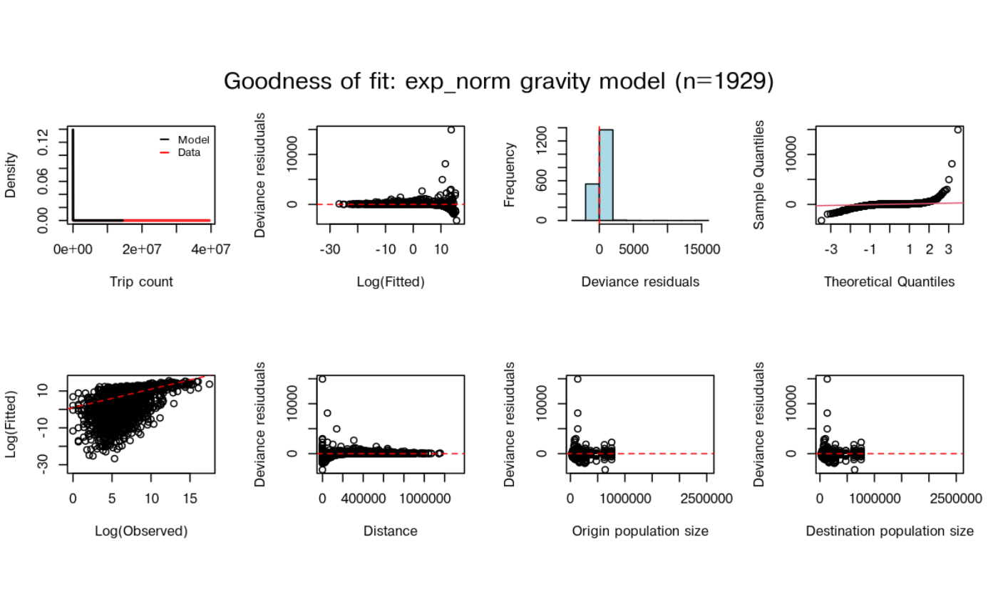
Prepare A Small Prediction Setting
To predict movement, we need a distance matrix D and a
population vector N for our regions. These are the same
inputs used by mobility::predict(). If the origins and
destinations have different populations, they can instead be supplied as
N_orig and N_dest.
Here we construct a small example with five place names. The populations and coordinates are invented to show how to arrange the inputs, and should not be used as estimates for those places. We multiply the distances between the coordinates by 120 to give our example distances in kilometres. For your own analysis, you could prepare these inputs from a shapefile and population data, as shown in the README example.
Show how to construct the example regions
places <- data.frame(
  name = c("Lusaka", "Kabwe", "Ndola", "Kitwe", "Livingstone"),
  x = c(0, 1.2, 2.8, 2.6, -1.4),
  y = c(0, 1.0, 2.7, 2.4, -2.7),
  population = c(2500000, 230000, 475000, 690000, 170000)
)

D <- as.matrix(dist(places[, c("x", "y")])) * 120
dimnames(D) <- list(places$name, places$name)
N <- setNames(places$population, places$name)
newdata <- list(D = D, N = N)
Make A Prediction
We can now pass the distances and populations to
predict(), specifying that our distances are in kilometres.
You will see warnings because these five regions contain a smaller
population and cover fewer locations than the data used to fit the
model. The prediction can still be calculated, but those warnings help
us identify differences between our example and the setting in which the
model was fit.
M <- predict(model, newdata = newdata, unit = "km")#> Warning: ! Prediction data have far fewer regions than the fitted source data.
#> ℹ `newdata` has "5" regions; the fitted model has "115".
#> • Predictions may be coarser than the source data can support.#> Warning: ! Prediction population is much smaller than the fitted source population.
#> ℹ `newdata` population: "4065000"; fitted model source population: "18296043".
#> • Check that this model is suitable for the population scale being predicted.
round(M / 1000, 1)#> Lusaka Kabwe Ndola Kitwe Livingstone
#> Lusaka 34681.3 53.7 0.0 0.0 0.1
#> Kabwe 4.9 3189.6 0.2 0.9 0.0
#> Ndola 0.0 0.3 5389.0 1210.3 0.0
#> Kitwe 0.0 2.1 1757.8 7826.9 0.0
#> Livingstone 0.0 0.0 0.0 0.0 2362.0
#> attr(,"model")
#> [1] "gravity"
#> attr(,"type")
#> [1] "exp_norm"
#> attr(,"source_duration_days")
#> [1] 21
#> attr(,"prediction_period_days")
#> [1] 21
#> attr(,"duration_scale")
#> [1] 1
#> attr(,"data_name")
#> [1] "zmb_fb_2025"The result is a matrix in which rows identify the origin of a trip
and columns identify its destination. We have divided the values by
1,000 to make them easier to read, so a value of 2 represents 2,000
predicted trips. These are counts of trips, to which a person may
contribute more than once. The period is taken from the model metadata
and is 21 days for this fit. The names on the distance matrix and
population vector must identify the same regions so that
nomad can match each population to the correct
location.
For a real analysis, we would now consider whether the model describes movement at a suitable scale for our question. For example, a model fit to movement between districts may tell us little about journeys between neighbourhoods within a city. Comparing alternatives is useful when several models could plausibly describe the movement we want to study.
Predict for the source regions
The fitted model also includes the distances and populations used for fitting. These inputs are often called covariates. We can reuse them to predict movement for the original regions, which provides a useful comparison with predictions for a new setting.
source_data <- model$get_model()$data[c("D", "N_orig", "N_dest")]
M_source <- predict(model, newdata = source_data)
M_source[1:5, 1:5]
#> destination
#> origin ZMB.1.1_1 ZMB.1.2_1 ZMB.1.3_1 ZMB.1.4_1 ZMB.1.5_1
#> ZMB.1.1_1 4.503207e+06 207404.91311 1.175758e+01 2.866407e+03 3.067882e+05
#> ZMB.1.2_1 4.595483e+04 997777.28396 2.401973e+01 4.359945e+01 1.965902e+05
#> ZMB.1.3_1 2.233465e+00 20.59288 8.554261e+05 1.436979e-03 3.196422e+01
#> ZMB.1.4_1 8.675690e+02 59.55731 2.289578e-03 1.362974e+06 5.927834e+01
#> ZMB.1.5_1 1.268509e+05 366863.60721 6.957575e+01 8.098131e+01 1.861987e+06Choose a prediction period
If we want a prediction for a different time period, we can supply
duration in days or a
date_start/date_end pair. This scales the
prediction in proportion to the period recorded in the model metadata,
assuming that the average daily trip rate stays constant. For example,
the request below uses 30 / 21 as its multiplier because the newer
Facebook models predict trip counts over 21 days. The dates over which
data were collected are stored separately and do not determine this
multiplier.
#> [1] 1.428571The returned duration_scale is the multiplier applied to
the original prediction, in this case approximately 1.43.
Models can also be shared through nomad with incomplete
source metadata, as with the earlier Zambia Facebook and CDR models from
2020. Without a prediction period, we can explore their unscaled
predictions but cannot convert the counts to trips over a specified
number of days. The package warns when returning such a prediction and
raises an error if we request a duration conversion. This makes the
available models accessible while showing where missing information
limits their use in an analysis.
Compare Alternatives
Several models were fit to the Zambia Facebook observations. We can
compare their fit statistics and use model_weights() to
calculate weights from one of those measures. Here we use root mean
squared error (RMSE), which gives more weight to models that reproduced
the source observations more closely. This comparison uses models fit to
the same dataset, so their errors refer to the same observed trips.
weights <- model_weights(data_name = "zmb_fb_2025", metric = "RMSE")
weights[, c("name", "RMSE", "weight")]
#> # A tibble: 12 × 3
#> name RMSE weight
#> <chr> <dbl> <dbl>
#> 1 zmb_fb_2025_mod_dd_exp 946018. 0.0898
#> 2 zmb_fb_2025_mod_dd_power 946521. 0.0897
#> 3 zmb_fb_2025_mod_dd_radiation 946973. 0.0897
#> 4 zmb_fb_2025_mod_grav_basic 819787890. 0.000104
#> 5 zmb_fb_2025_mod_grav_exp 947086. 0.0897
#> 6 zmb_fb_2025_mod_grav_exp_norm 965442. 0.0879
#> 7 zmb_fb_2025_mod_grav_power 942100. 0.0901
#> 8 zmb_fb_2025_mod_grav_power_norm 946881. 0.0897
#> 9 zmb_fb_2025_mod_grav_scaled_power 952655. 0.0891
#> 10 zmb_fb_2025_mod_grav_transport 1057907. 0.0803
#> 11 zmb_fb_2025_mod_rad_basic 831656. 0.102
#> 12 zmb_fb_2025_mod_rad_finite 833482. 0.102We can also use nomad_ensemble() to combine predictions
from several models. For a simple example, we will select the
exponential departure-diffusion model and combine it with the gravity
model used above. Both were fit to the same Facebook dataset. Because we
ask each model to predict for the same regions and period, we can take a
weighted average of their predicted trip counts. We choose weights of
0.5 for this example, giving each model equal influence, rather than
deriving the weights from their fit statistics.
departure_model <- model_db$zmb_fb_2025_mod_dd_exp
ensemble <- nomad_ensemble(
  list(departure = departure_model, gravity = model),
  weights = c(departure = 0.5, gravity = 0.5)
)
M_ensemble <- predict(ensemble, newdata = newdata, unit = "km")
#> Warning: ! Prediction data have far fewer regions than the fitted source data.
#> ℹ `newdata` has "5" regions; the fitted model has "115".
#> • Predictions may be coarser than the source data can support.#> Warning: ! Prediction population is much smaller than the fitted source population.
#> ℹ `newdata` population: "4065000"; fitted model source population: "18296043".
#> • Check that this model is suitable for the population scale being predicted.#> Warning: ! Prediction data have far fewer regions than the fitted source data.
#> ℹ `newdata` has "5" regions; the fitted model has "115".
#> • Predictions may be coarser than the source data can support.#> Warning: ! Prediction population is much smaller than the fitted source population.
#> ℹ `newdata` population: "4065000"; fitted model source population: "18296043".
#> • Check that this model is suitable for the population scale being predicted.#> [1] 56989960Explore parameter uncertainty
So far we have used the mean fitted parameters to make each
prediction. Setting nsim to a value greater than one
instead gives repeated predictions using approximate parameter draws
from the stored means and standard deviations. The summary below reports
how much the total number of trips and the number between different
regions vary across those draws. This captures parameter uncertainty
within the selected model, while comparing alternative models lets us
explore uncertainty about the choice of model itself.
draws <- predict(model, newdata = source_data, nsim = 10, seed = 1)
uncertainty_summary(draws, metrics = c("total", "between_region"))
#> # A tibble: 6 × 3
#> metric prob value
#> <chr> <dbl> <dbl>
#> 1 total 0.025 254163766.
#> 2 total 0.5 254206733.
#> 3 total 0.975 254234581.
#> 4 between_region 0.025 93395200.
#> 5 between_region 0.5 93420244.
#> 6 between_region 0.975 93436944.To explore these choices further, Selecting a mobility model works through the warnings and uncertainty summaries in more detail, and shows how to compare predictions from several models. Once you have a set of plausible models, Identifying a mobility model for an outbreak shows how to compare them using the daily incidence of a simulated outbreak.