Why This Workflow?
This vignette uses the same shared case-study object as the fitting vignette, then compares four paper-style intervention scenarios in one coherent view:
- Baseline response.
- Anticipatory action.
- Anticipatory action plus one vaccine dose.
- Anticipatory action plus two vaccine doses.
library(chlaa)
library(ggplot2)
library(dplyr)
#>
#> Attaching package: 'dplyr'
#> The following objects are masked from 'package:stats':
#>
#>     filter, lag
#> The following objects are masked from 'package:base':
#>
#>     intersect, setdiff, setequal, union

case_study <- chlaa_case_study_setup(seed = 42)
pars <- case_study$pars
scenarios <- case_study$scenarios
time <- case_study$time

vapply(scenarios, `[[`, character(1), "name")
#> [1] "scenario_1_baseline"
#> [2] "scenario_2_anticipatory_action"
#> [3] "scenario_3_anticipatory_action_plus_one_vaccine_dose"
#> [4] "scenario_4_anticipatory_action_plus_two_vaccine_doses"
1) Run The Scenario Set
runs <- chlaa_run_scenarios(
  pars = pars,
  scenarios = scenarios,
  time = time,
  n_particles = 40,
  dt = 1,
  seed = 1
)
2) Plot Infection-Rate Trajectories Together
plot_df <- runs |>
  group_by(scenario, time) |>
  summarise(infections_per_day = mean(inc_infections), .groups = "drop") |>
  mutate(
    date = case_study$dates$start_date + time,
    infections_k = infections_per_day / 1000
  )

label_map <- c(
  scenario_1_baseline = "Scenario 1: baseline",
  scenario_2_anticipatory_action = "Scenario 2: anticipatory action",
  scenario_3_anticipatory_action_plus_one_vaccine_dose = "Scenario 3: anticipatory action plus one vaccine dose",
  scenario_4_anticipatory_action_plus_two_vaccine_doses = "Scenario 4: anticipatory action plus two vaccine doses"
)

plot_df$scenario_label <- label_map[plot_df$scenario]

trigger_date <- case_study$dates$trigger_date
declaration_date <- case_study$dates$declaration_date

# Style mirrors the paper-like comparison: all scenarios together,
# intervention timing marked, and infection rates shown in thousands/day.
ggplot(plot_df, aes(x = date, y = infections_k, colour = scenario_label, linetype = scenario_label)) +
  geom_line(linewidth = 0.8) +
  geom_vline(xintercept = as.numeric(trigger_date), colour = "grey40") +
  geom_vline(xintercept = as.numeric(declaration_date), colour = "grey40") +
  annotate("text", x = trigger_date, y = max(plot_df$infections_k) * 0.9, label = "AA trigger", angle = 90, vjust = -0.3, size = 3) +
  annotate("text", x = declaration_date, y = max(plot_df$infections_k) * 0.9, label = "Outbreak declaration", angle = 90, vjust = -0.3, size = 3) +
  scale_colour_manual(values = c(
    "Scenario 1: baseline" = "#7f0000",
    "Scenario 2: anticipatory action" = "#b04a2f",
    "Scenario 3: anticipatory action plus one vaccine dose" = "#7d2d2d",
    "Scenario 4: anticipatory action plus two vaccine doses" = "#c15a40"
  )) +
  scale_linetype_manual(values = c(
    "Scenario 1: baseline" = "solid",
    "Scenario 2: anticipatory action" = "11",
    "Scenario 3: anticipatory action plus one vaccine dose" = "dotted",
    "Scenario 4: anticipatory action plus two vaccine doses" = "longdash"
  )) +
  labs(
    x = "Date",
    y = "Infection rate (persons/day x 10^3)",
    colour = "Intervention scenario",
    linetype = "Intervention scenario",
    title = "Scenario infection-rate trajectories"
  ) +
  theme_minimal()
#> Warning in scale_x_date(): A <numeric> value was passed to a Date scale.
#> ℹ The value was converted to a <Date> object.
#> A <numeric> value was passed to a Date scale.
#> ℹ The value was converted to a <Date> object.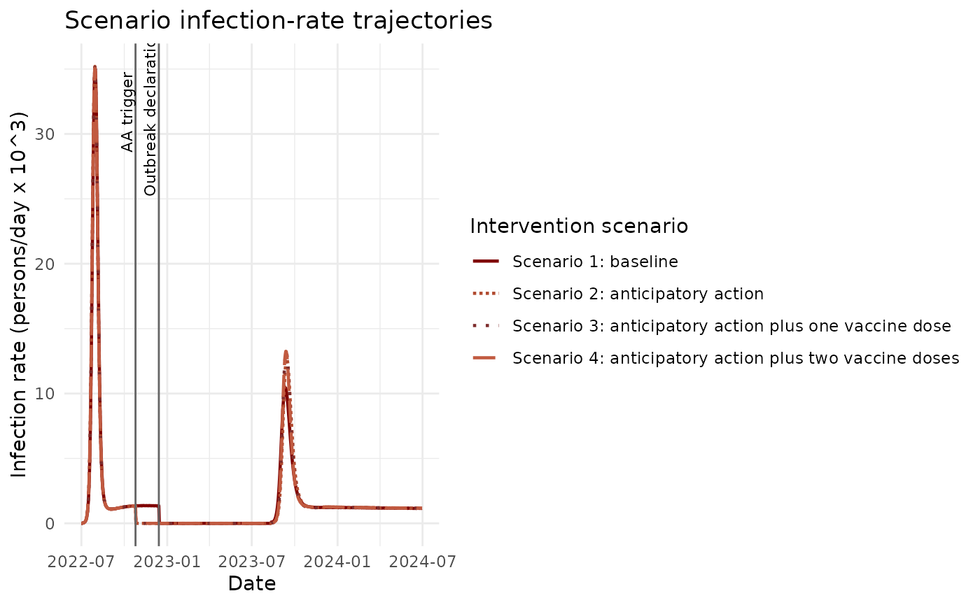
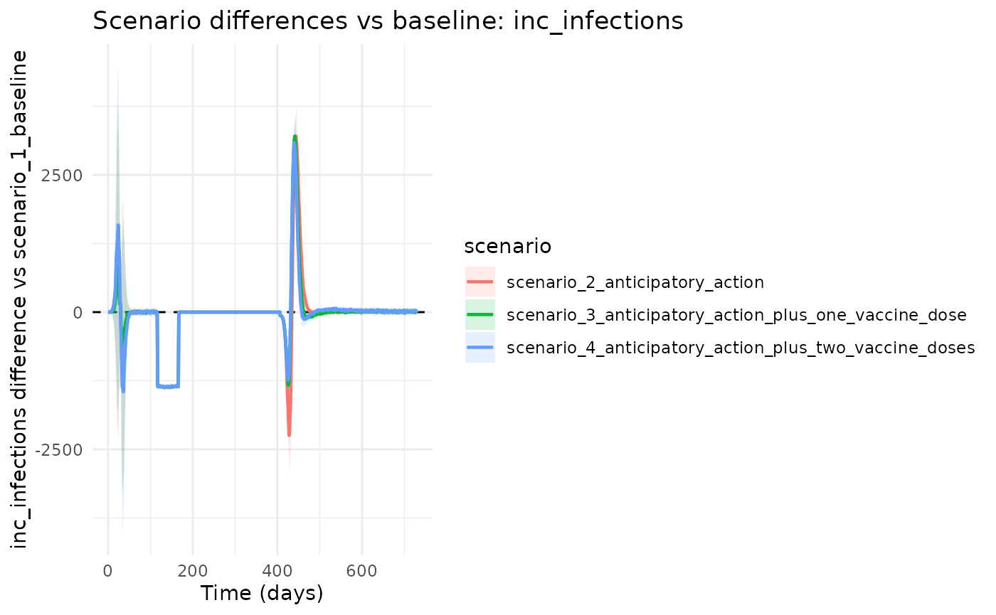
3) Plot Differences Versus Baseline
chlaa_plot_difference_vs_baseline(
  runs,
  baseline = "scenario_1_baseline",
  var = "inc_infections",
  cumulative = FALSE
)
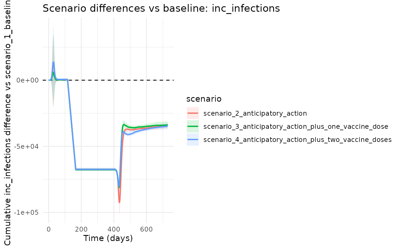
chlaa_plot_difference_vs_baseline(
  runs,
  baseline = "scenario_1_baseline",
  var = "inc_infections",
  cumulative = TRUE
)
4) Decision-Facing Summary Tables
summary_tbl <- chlaa_scenario_summary(runs, baseline = "scenario_1_baseline", incidence_var = "inc_infections")
summary_tbl
#> # A tibble: 4 × 8
#>   scenario  total_cases total_deaths cases_averted deaths_averted peak_incidence
#>   <chr>           <dbl>        <dbl>         <dbl>          <dbl>          <dbl>
#> 1 scenario…     320787.       47343.            0              0          35252.
#> 2 scenario…     312255.       46044.         8531.          1300.         35285.
#> 3 scenario…     312461.       46109.         8325.          1234.         35292.
#> 4 scenario…     312174.       46000.         8612.          1343.         35285.
#> # ℹ 2 more variables: time_peak <dbl>, time_to_control <dbl>
cmp <- chlaa_compare_scenarios(
  runs,
  baseline = "scenario_1_baseline",
  include_econ = TRUE,
  wtp = 1500
)
cmp
#> # A tibble: 4 × 21
#>   scenario    infections cases_symptomatic deaths  doses orc_treated ctc_treated
#>   <chr>            <dbl>             <dbl>  <dbl>  <dbl>       <dbl>       <dbl>
#> 1 scenario_1…   1289454.           320787. 47343. 2.80e5        164.        141.
#> 2 scenario_2…   1254669.           312255. 46044. 2.80e5        163.        137.
#> 3 scenario_3…   1255906.           312461. 46109. 2.80e5        163.        140.
#> 4 scenario_4…   1254725.           312174. 46000. 1.79e5        166.        140.
#> # ℹ 14 more variables: infections_averted <dbl>, cases_averted <dbl>,
#> #   deaths_averted <dbl>, cost <dbl>, dalys <dbl>, cost_diff <dbl>,
#> #   dalys_averted <dbl>, icer_cost_per_daly_averted <dbl>,
#> #   icer_cost_per_death_averted <dbl>, mean_cost_vax <dbl>,
#> #   mean_cost_care <dbl>, mean_cost_wash <dbl>, nmb <dbl>, inmb <dbl>