Why This Workflow?
This vignette fits the model to a cleaned historical outbreak time series digitized from Fig. 3 in:
Milano et al. (2025), modelling cholera response in the Democratic Republic of the Congo.
The cleaned series is bundled in the package so the workflow is fully reproducible.
library(chlaa)
library(ggplot2)

data_path <- system.file(
  "extdata", "outbreak", "nyiragongo_historical_cases_clean.csv",
  package = "chlaa"
)
stopifnot(nzchar(data_path))

example_data <- read.csv(data_path, stringsAsFactors = FALSE)
example_data$date <- as.Date(example_data$date)
example_data$time <- as.integer(example_data$date - min(example_data$date))

# Keep shared baseline parameterization for a stable CI example fit.
case_study <- chlaa_case_study_setup(seed = 42)

head(example_data)
#>         date cases
#> 1 2022-08-01     6
#> 2 2022-08-02     6
#> 3 2022-08-03     6
#> 4 2022-08-04     7
#> 5 2022-08-05     7
#> 6 2022-08-06     7
#>                                                                source time
#> 1 Milano et al. (2025) Fig. 3 historical data (digitized and cleaned)    0
#> 2 Milano et al. (2025) Fig. 3 historical data (digitized and cleaned)    1
#> 3 Milano et al. (2025) Fig. 3 historical data (digitized and cleaned)    2
#> 4 Milano et al. (2025) Fig. 3 historical data (digitized and cleaned)    3
#> 5 Milano et al. (2025) Fig. 3 historical data (digitized and cleaned)    4
#> 6 Milano et al. (2025) Fig. 3 historical data (digitized and cleaned)    5
1) Visualise The Shared Outbreak Data
ggplot(example_data, aes(x = date, y = cases)) +
  geom_line(linewidth = 0.5, colour = "black") +
  labs(
    x = "Date",
    y = "Reported cholera cases/day",
    title = "Cleaned historical outbreak data (Milano et al. Fig. 3)"
  ) +
  theme_minimal()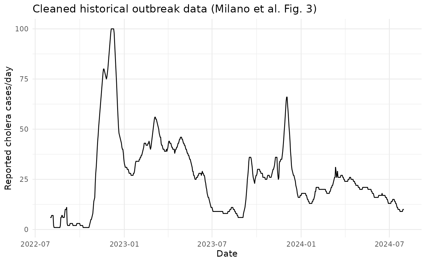
2) Prepare Data And Starting Parameters
To keep vignette runtime practical on CI, we fit an early-to-mid outbreak window and reserve later dynamics for scenario/economic workflows.
fit_data_raw <- subset(example_data, date <= as.Date("2023-06-30"))
fit_data <- chlaa_prepare_data(fit_data_raw, time_col = "time", cases_col = "cases")

pars_start <- case_study$pars
pars_start$Sev0 <- 20
pars_start$E0 <- 20
pars_start$M0 <- 10
pars_start$contact_rate <- pars_start$contact_rate * 0.95
pars_start$trans_prob <- pars_start$trans_prob * 1.05
pars_start$reporting_rate <- 0.20
pars_start$obs_size <- 30
3) Fit With pMCMC
fit <- chlaa_fit_pmcmc(
data = fit_data,
pars = pars_start,
n_particles = 60,
n_steps = 260,
seed = 42,
proposal_var = 1e-5
)
#> ⡀⠀ Sampling ■ | 0% ETA: 15s
#> ⠄⠀ Sampling ■■■■■■ | 16% ETA: 5s
#> ⢂⠀ Sampling ■■■■■■■■■■■■■■■■■■■■■■ | 69% ETA: 2s
#> ✔ Sampled 260 steps across 1 chain in 5.7s
#>
fit
#> <chlaa_fit>
#> Posterior draws: 260 iterations; 9 parameters
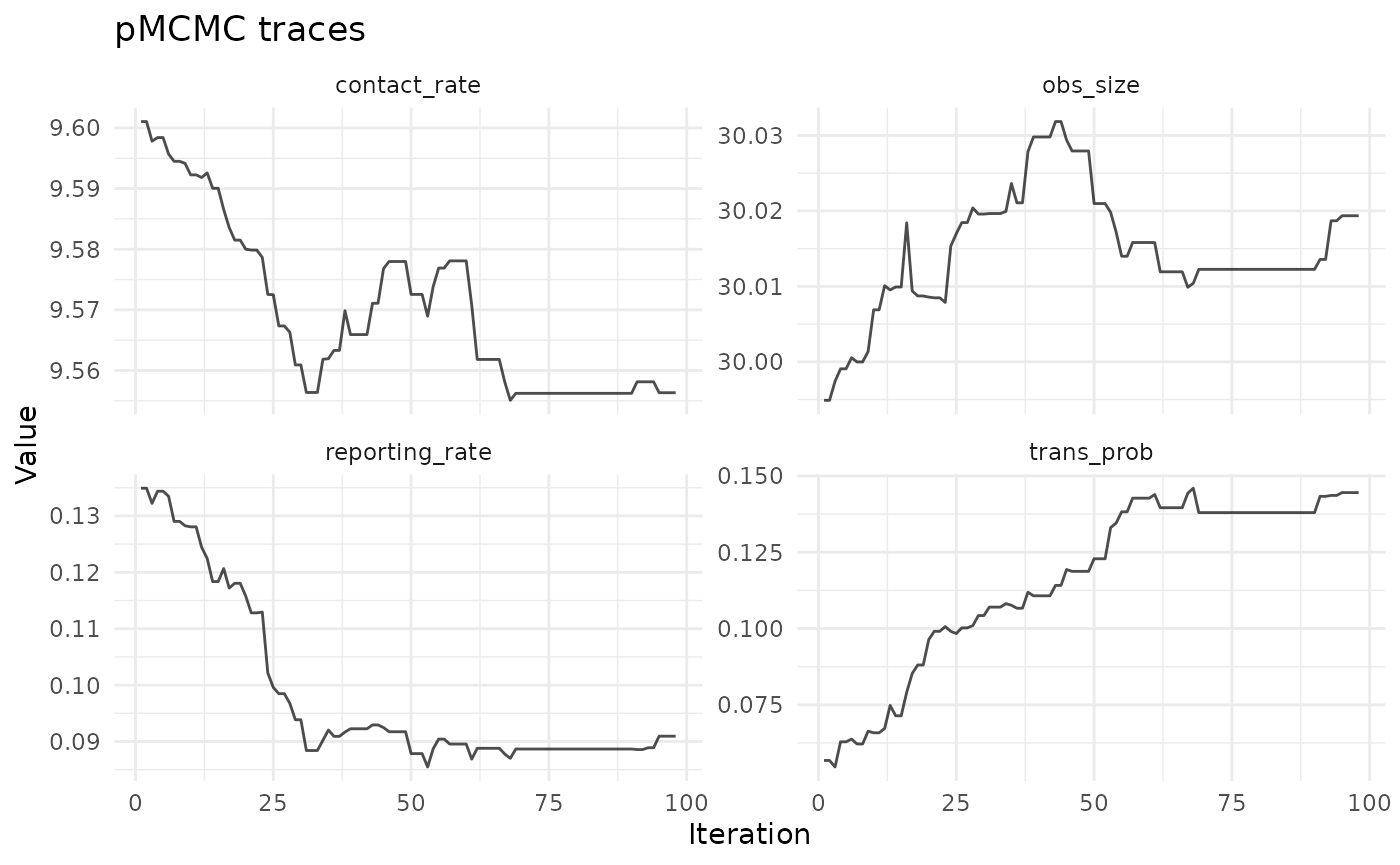
#> Data: 334 observations; time range [0, 333]4) Diagnostics
fit_report <- chlaa_fit_report(fit, burnin = 0.25, thin = 2)
fit_report$acceptance_rate
#> [1] 0.4329897
chlaa_plot_trace(
  fit,
  parameters = c("trans_prob", "contact_rate", "reporting_rate", "obs_size"),
  burnin = 0.25,
  thin = 2
)
chlaa_plot_likelihood_trace(fit, burnin = 0.25, thin = 2)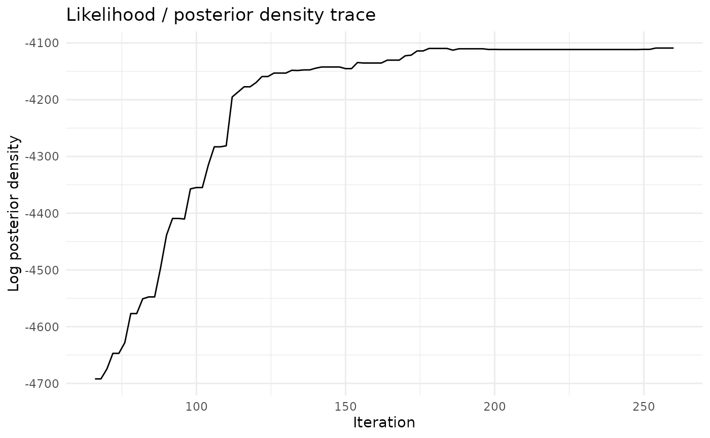
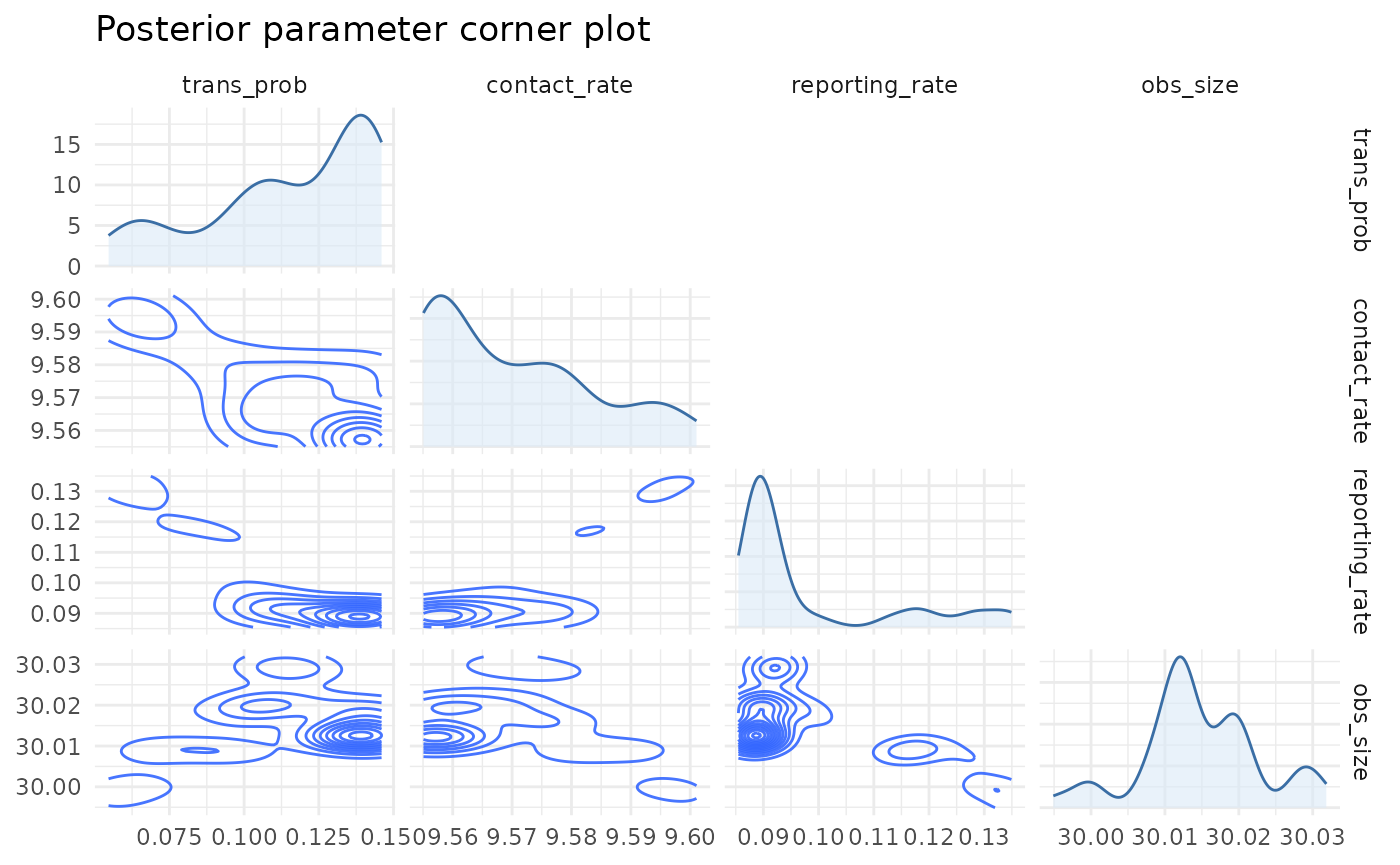
chlaa_plot_parameter_pairs(
  fit,
  parameters = c("trans_prob", "contact_rate", "reporting_rate", "obs_size"),
  burnin = 0.25,
  thin = 2,
  max_points = 1500
)
chlaa_plot_parameter_vs_likelihood(
  fit,
  parameters = c("trans_prob", "contact_rate", "reporting_rate"),
  burnin = 0.25,
  thin = 2,
  max_points = 1500
)
#> `geom_smooth()` using method = 'loess' and formula = 'y ~ x'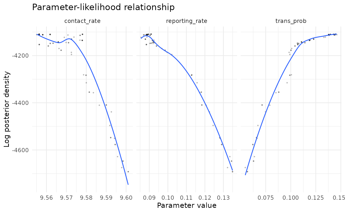
5) Posterior Predictive Projection
start_date <- min(example_data$date)
forecast_end <- as.Date("2024-09-30")
forecast_time <- 0:as.integer(forecast_end - start_date)

fc <- chlaa_forecast_from_fit(
  fit = fit,
  pars = pars_start,
  time = forecast_time,
  vars = "inc_symptoms",
  include_cases = TRUE,
  quantiles = c(0.025, 0.125, 0.25, 0.5, 0.75, 0.875, 0.975),
  n_draws = 80,
  burnin = 0.25,
  thin = 2,
  seed = 42,
  dt = 1,
  n_particles = 1
)

f_cases <- fc[fc$variable == "cases", ]
f_cases$date <- start_date + f_cases$time

obs <- example_data

# Overlay style mirrors the narrative used in the paper figures:
# historical line, mean projection, and nested uncertainty bands.
ggplot() +
  geom_line(data = obs, aes(x = date, y = cases, colour = "Historical data"), linewidth = 0.5) +
  geom_line(data = f_cases, aes(x = date, y = mean, colour = "Mean projection"), linewidth = 0.7) +
  geom_line(data = f_cases, aes(x = date, y = q0p25, colour = "50% UI"), linewidth = 0.5) +
  geom_line(data = f_cases, aes(x = date, y = q0p75, colour = "50% UI"), linewidth = 0.5) +
  geom_line(data = f_cases, aes(x = date, y = q0p125, colour = "75% UI"), linewidth = 0.4, linetype = 2) +
  geom_line(data = f_cases, aes(x = date, y = q0p875, colour = "75% UI"), linewidth = 0.4, linetype = 2) +
  geom_line(data = f_cases, aes(x = date, y = q0p025, colour = "95% UI"), linewidth = 0.4) +
  geom_line(data = f_cases, aes(x = date, y = q0p975, colour = "95% UI"), linewidth = 0.4) +
  scale_colour_manual(values = c(
    "Historical data" = "black",
    "Mean projection" = "#2c7f62",
    "50% UI" = "#b88a66",
    "75% UI" = "#8c8c8c",
    "95% UI" = "#9a3b32"
  )) +
  labs(
    x = "Date",
    y = "Reported cholera cases/day",
    colour = NULL,
    title = "Historical data and fitted model projection"
  ) +
  theme_minimal()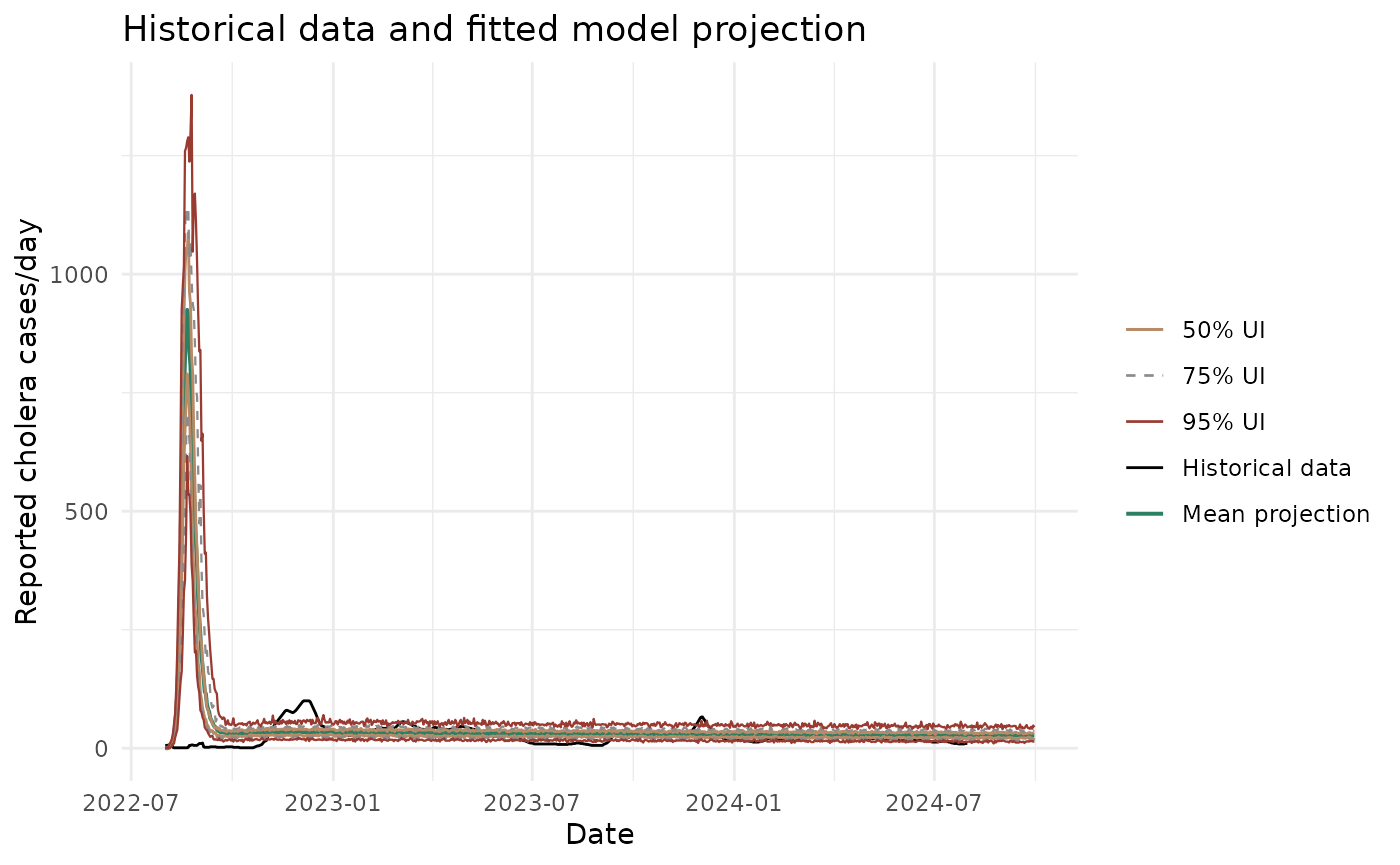
Interpretation
This fitting run is intentionally compact to stay CI-friendly while still showing the full workflow. For substantive analyses, increase chain length, particles, and number of seeds, and carry posterior uncertainty through counterfactual and economic decision analysis. Because the observed data are now paper-derived, the fitted trajectory should resemble the historical outbreak shape shown in Milano et al. more closely than synthetic examples.