Health Economics and Optimisation
Source:vignettes/health_econ_and_optimisation.Rmd
health_econ_and_optimisation.RmdWhy This Workflow?
This vignette uses the same case-study data and scenario assumptions as the fitting and scenario vignettes, then extends to economic comparison and budget allocation.
Compared with the earlier version, this workflow includes a richer scenario set, explicit source metadata, and multiple decision-support plots.
library(chlaa)
library(ggplot2)
library(dplyr)
#>
#> Attaching package: 'dplyr'
#> The following objects are masked from 'package:stats':
#>
#>     filter, lag
#> The following objects are masked from 'package:base':
#>
#>     intersect, setdiff, setequal, union

case_study <- chlaa_case_study_setup(seed = 42)
pars <- case_study$pars
time <- case_study$time

base_scenarios <- case_study$scenarios
1) Build An Expanded Scenario Set
We add no-vaccine comparators to make the economic frontier more informative.
strip_vax <- function(mod) {
  out <- mod
  out$vax1_start <- 0
  out$vax1_end <- 0
  out$vax1_total_doses <- 0
  out$vax1_doses_per_day <- 0
  out$vax2_start <- 0
  out$vax2_end <- 0
  out$vax2_total_doses <- 0
  out$vax2_doses_per_day <- 0
  out
}

scenario_5 <- chlaa_scenario(
  "scenario_5_baseline_response_no_vaccine",
  strip_vax(base_scenarios[[1]]$modify)
)

scenario_6 <- chlaa_scenario(
  "scenario_6_anticipatory_action_no_vaccine",
  strip_vax(base_scenarios[[2]]$modify)
)

scenarios <- c(base_scenarios, list(scenario_5, scenario_6))

runs <- chlaa_run_scenarios(
  pars = pars,
  scenarios = scenarios,
  time = time,
  n_particles = 40,
  dt = 1,
  seed = 2
)
2) Economics Assumptions And Sources
econ <- chlaa_econ_defaults()
econ_sources <- chlaa_econ_sources()

head(econ_sources)
#>                                        name
#> cost_per_vaccine_dose             published
#> cost_per_orc_treatment           assumption
#> cost_per_ctc_treatment           assumption
#> cost_chlorination_per_person_day assumption
#> cost_hygiene_per_person_day      assumption
#> cost_latrine_per_person_day      assumption
#>                                                                                                                            source_type
#> cost_per_vaccine_dose            Routh et al. (2017) Cost Evaluation of a Government-Conducted Oral Cholera Vaccination Campaign—Haiti
#> cost_per_orc_treatment                                                    Illustrative planning assumption for rapid scenario analysis
#> cost_per_ctc_treatment                                                    Illustrative planning assumption for rapid scenario analysis
#> cost_chlorination_per_person_day                                          Illustrative planning assumption for rapid scenario analysis
#> cost_hygiene_per_person_day                                               Illustrative planning assumption for rapid scenario analysis
#> cost_latrine_per_person_day                                               Illustrative planning assumption for rapid scenario analysis
#>                                  citation
#> cost_per_vaccine_dose                2013
#> cost_per_orc_treatment
#> cost_per_ctc_treatment
#> cost_chlorination_per_person_day
#> cost_hygiene_per_person_day
#> cost_latrine_per_person_day
#>                                                                                                                            source_url
#> cost_per_vaccine_dose                                                               https://pmc.ncbi.nlm.nih.gov/articles/PMC5676633/
#> cost_per_orc_treatment           No single globally transferable unit cost; should be replaced with context-specific ORS/ORC costing.
#> cost_per_ctc_treatment                          No single globally transferable unit cost; should be replaced with local CTC costing.
#> cost_chlorination_per_person_day                                 WASH package unit costs vary widely by programme design and context.
#> cost_hygiene_per_person_day                                      WASH package unit costs vary widely by programme design and context.
#> cost_latrine_per_person_day                                      WASH package unit costs vary widely by programme design and context.
#>                                                                                                                                 notes
#> cost_per_vaccine_dose            Total campaign cost per dose around USD 2.90 in Haiti 2013; default uses rounded illustrative value.
#> cost_per_orc_treatment
#> cost_per_ctc_treatment
#> cost_chlorination_per_person_day
#> cost_hygiene_per_person_day
#> cost_latrine_per_person_day
subset(econ_sources, source_type == "published")
#> [1] name        source_type citation    source_url  notes
#> <0 rows> (or 0-length row.names)
3) Incremental Cost-Effectiveness Table
cmp <- chlaa_compare_scenarios(
  runs,
  baseline = "scenario_1_baseline",
  include_econ = TRUE,
  econ = econ,
  wtp = 1500
)
cmp
#> # A tibble: 6 × 21
#>   scenario    infections cases_symptomatic deaths  doses orc_treated ctc_treated
#>   <chr>            <dbl>             <dbl>  <dbl>  <dbl>       <dbl>       <dbl>
#> 1 scenario_1…   1289598.           320902. 47372  2.80e5        163.        141.
#> 2 scenario_2…   1254692.           312228. 46052. 2.80e5        163.        140.
#> 3 scenario_3…   1255735.           312434. 46034. 2.80e5        166.        140.
#> 4 scenario_4…   1254721            312100. 45990. 1.79e5        163.        141.
#> 5 scenario_5…   1292961.           321517. 47426. 0             165.        139.
#> 6 scenario_6…   1258280.           312812. 46101. 0             162.        137.
#> # ℹ 14 more variables: infections_averted <dbl>, cases_averted <dbl>,
#> #   deaths_averted <dbl>, cost <dbl>, dalys <dbl>, cost_diff <dbl>,
#> #   dalys_averted <dbl>, icer_cost_per_daly_averted <dbl>,
#> #   icer_cost_per_death_averted <dbl>, mean_cost_vax <dbl>,
#> #   mean_cost_care <dbl>, mean_cost_wash <dbl>, nmb <dbl>, inmb <dbl>
4) Visualise Incremental Outcomes
plot_cmp <- cmp |>
  mutate(
    scenario = factor(scenario, levels = scenario),
    deaths_averted_vs_baseline = deaths_averted
  )

ggplot(plot_cmp, aes(x = scenario, y = deaths_averted_vs_baseline, fill = scenario)) +
  geom_col(show.legend = FALSE) +
  coord_flip() +
  labs(
    x = NULL,
    y = "Deaths averted vs scenario_1_baseline",
    title = "Incremental health benefit across expanded scenario set"
  ) +
  theme_minimal()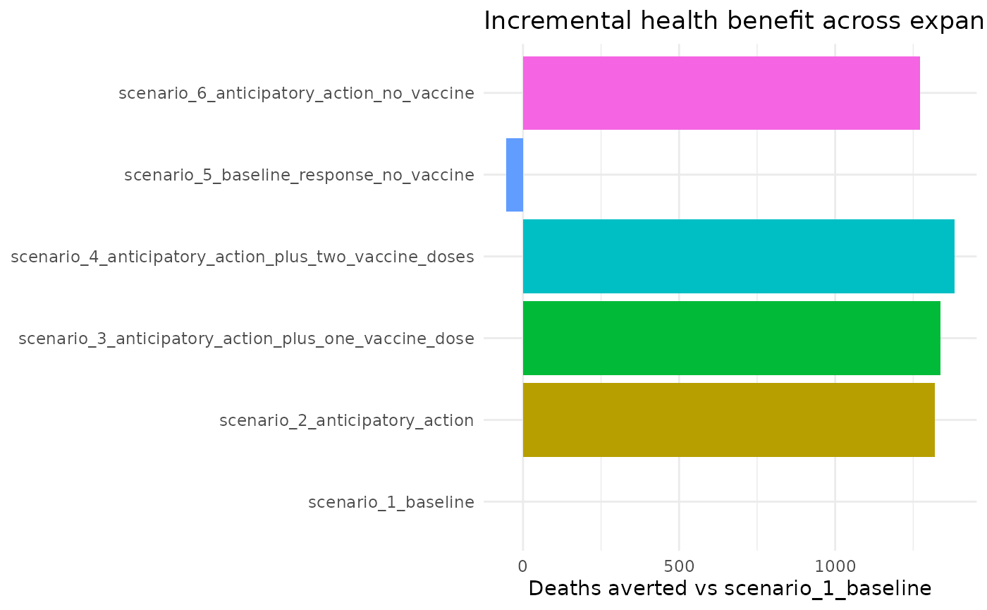
chlaa_plot_ce_plane(cmp)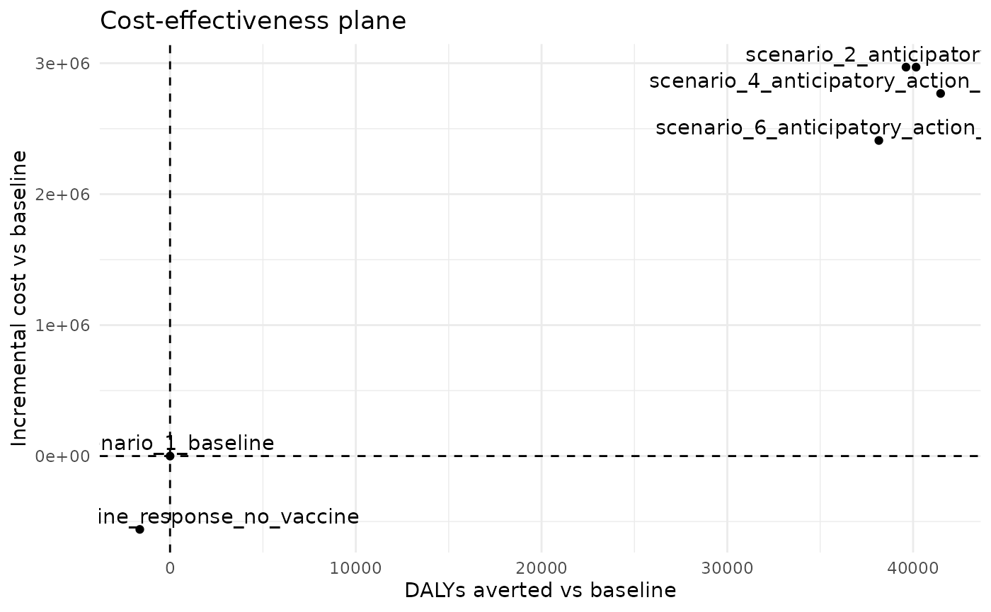
5) CEAC With Expanded Scenario Set
ceac_tbl <- chlaa_ceac(
  runs,
  baseline = "scenario_1_baseline",
  wtp = seq(0, 3000, by = 250),
  econ = econ
)

head(ceac_tbl)
#> # A tibble: 6 × 3
#>   scenario                                                wtp prob_best
#>   <chr>                                                 <dbl>     <dbl>
#> 1 scenario_5_baseline_response_no_vaccine                   0     1
#> 2 scenario_2_anticipatory_action                          250     0.25
#> 3 scenario_3_anticipatory_action_plus_one_vaccine_dose    250     0.275
#> 4 scenario_4_anticipatory_action_plus_two_vaccine_doses   250     0.275
#> 5 scenario_6_anticipatory_action_no_vaccine               250     0.2
#> 6 scenario_2_anticipatory_action                          500     0.25
ggplot(ceac_tbl, aes(x = wtp, y = prob_best, colour = scenario)) +
  geom_line(linewidth = 0.8) +
  labs(
    x = "WTP (USD per DALY averted)",
    y = "Probability cost-effective",
    colour = "Scenario",
    title = "Cost-effectiveness acceptability curves"
  ) +
  theme_minimal()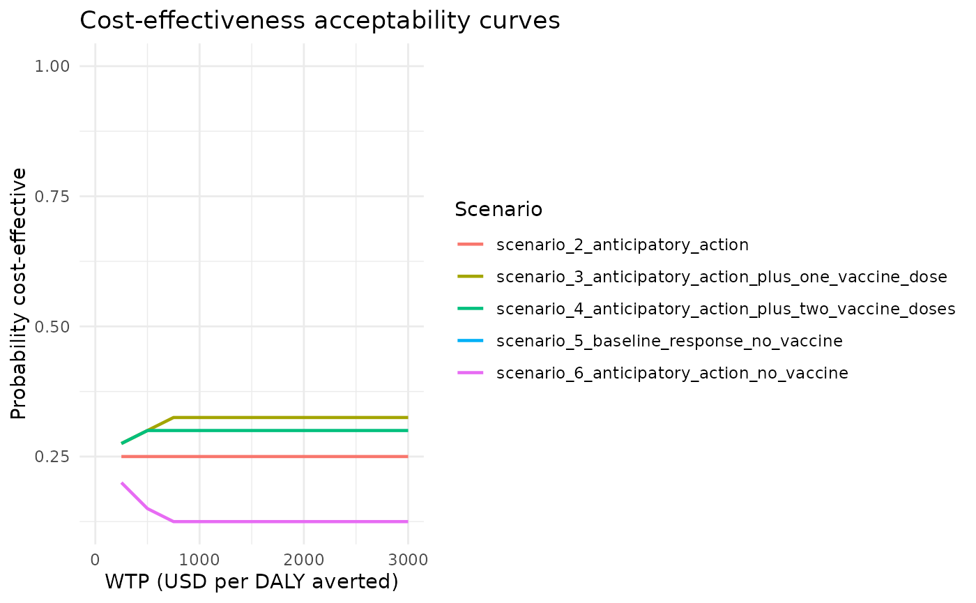
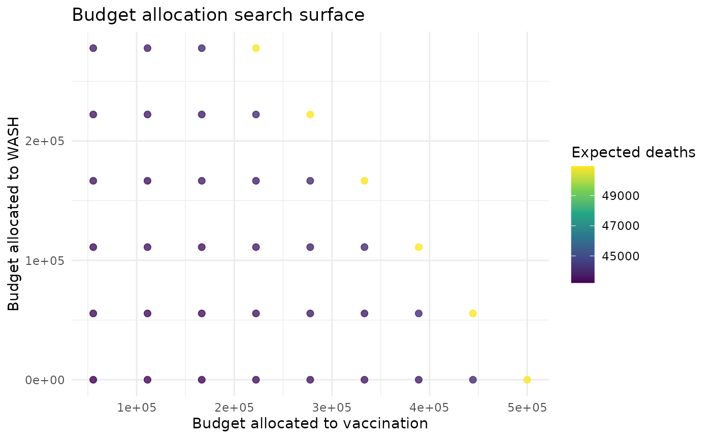
6) Budget Allocation Optimisation
opt <- chlaa_optimise_budget(
  pars = pars,
  budget = 5e5,
  time = time,
  n_particles = 20,
  dt = 1,
  grid_size = 10,
  min_fraction = list(vax = 0.1),
  max_fraction = list(wash = 0.6),
  max_vax_doses_per_day = 5000
)

opt$best
#>    frac_vax frac_wash frac_care budget_vax budget_wash budget_care doses
#> 1 0.1111111         0 0.8888889   55555.56           0    444444.4 27777
#>   wash_intensity   deaths    cases
#> 1              0 43215.75 344971.2
ggplot(opt$evaluations, aes(x = budget_vax, y = budget_wash, colour = deaths)) +
  geom_point(size = 2, alpha = 0.8) +
  scale_colour_viridis_c() +
  labs(
    x = "Budget allocated to vaccination",
    y = "Budget allocated to WASH",
    colour = "Expected deaths",
    title = "Budget allocation search surface"
  ) +
  theme_minimal()