Model output, loggers and saved state
OJ Watson
2026-11-11
Source:vignettes/Loggers.Rmd
Loggers.RmdOverview
A magenta simulation holds its entire state in C++
memory. What comes back into R is whatever you ask
pipeline() to extract, and the choice matters: a full
population dump at monthly intervals over 40 years is large enough to be
awkward, while the default summary may not contain what you need.
This vignette describes what each saving option returns, what the individual loggers mean, and how to save a simulation to disk and restart it later.
The default: loggers only
With no saving options, pipeline() runs to the end and
returns a single list containing Loggers, a snapshot of the
population at the final time step.
out <- pipeline(EIR = 5, N = 1000, years = 3, ft = 0.4, seed = 1L)
## Seed set to 1
## magenta v1.3.7
names(out$Loggers)
##  [1] "Log_Counter"              "Incidence"
##  [3] "Incidence_05"             "Treatments"
##  [5] "daily_mutations_per_loci" "InfectionStates"
##  [7] "Ages"                     "IB"
##  [9] "ICA"                      "ICM"
## [11] "ID"                       "Mosquitoes"
## [13] "Time"                     "S"
## [15] "D"                        "A"
## [17] "U"                        "T"
## [19] "P"
The entries fall into four groups.
Population state. S, D,
A, U, T and P are
the proportion of people in each infection state: susceptible, clinical
disease, asymptomatic, subpatent, treated and prophylactic.
as.data.frame(out$Loggers[c("S", "D", "A", "U", "T", "P")])
##           S           D         A         U           T          P
## 1 0.6158804 0.003590868 0.2853543 0.0826347 0.002294064 0.01024566
Per individual vectors. Ages (in days),
InfectionStates coded 0:5 in the order above,
and the four immunity functions: IB (pre-erythrocytic),
ICA (acquired clinical), ICM (maternal
clinical) and ID (detection). ID is the one
used to decide whether an infection would be detected by microscopy, and
is needed by convert_barcode_vectors().
sapply(out$Loggers[c("Ages", "InfectionStates", "IB", "ICA", "ICM", "ID")], length)
##            Ages InfectionStates              IB             ICA             ICM
##            1000            1000            1000            1000            1000
##              ID
##            1000
Counters. Incidence and
Incidence_05 are clinical cases over the logging window,
all ages and under fives respectively. Log_Counter is the
number of days that window covered, which is what you divide by to turn
counts into rates. daily_mutations_per_loci counts
mutations at each barcode locus.
Sub-lists. Treatments records treatment
outcomes and biting:
str(out$Loggers$Treatments)
## List of 5
##  $ Successful_Treatments         : num 448
##  $ Unsuccesful_Treatments_LPF    : num 0
##  $ Not_Treated                   : num 690
##  $ daily_bite_counters           : int 972234
##  $ daily_infectious_bite_counters: int 10231
Successful_Treatments and
Unsuccesful_Treatments_LPF are counts of treatments that
cured and that ended in a 28 day late parasitological failure. With more
than one drug deployed these become vectors, one entry per drug.
Not_Treated counts clinical cases that did not receive
treatment. daily_bite_counters and
daily_infectious_bite_counters accumulate bites over the
logging window, and dividing the latter by Log_Counter and
the population size gives the EIR.
Mosquitoes holds the vector population in each state,
and is populated when the simulation is run with update saves:
out_u <- pipeline(EIR = 5, N = 1000, years = 3, ft = 0.4, seed = 1L,
                  update_save = TRUE, update_length = 90)
## Seed set to 1
## magenta v1.3.7
## Starting Stochastic Simulation for 3 years
str(out_u[[1]]$Mosquitoes)
## List of 3
##  $ Mos_S: num 2775
##  $ Mos_E: num 91.3
##  $ Mos_I: num 34.2
Saving through time
update_save = TRUE stops the simulation every
update_length days, extracts a summary, and carries on. The
result is a list with one element per interval.
length(out_u)
## [1] 12
3 * 365 / 90
## [1] 12.16667
The final element is not a summary. It holds the simulation object itself, so that the run can be continued or interrogated. Every piece of code that loops over the output therefore needs to drop it:
pos <- seq_len(length(out_u) - 1)
prev <- unlist(lapply(out_u[pos], function(x) sum(unlist(x[c("D", "A", "U", "T")]))))
time <- unlist(lapply(out_u[pos], "[[", "Time"))
plot(time / 365, prev, type = "l", lwd = 2, col = "steelblue",
     xlab = "Years", ylab = "PCR prevalence", ylim = c(0, max(prev)))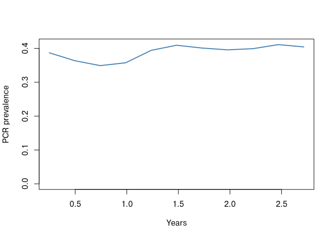
Reproducibility metadata
Every returned object carries a meta attribute holding
the call, the seed and the package version. Keep this: it is the record
of how a simulation was produced.
meta <- attr(out_u, "meta")
meta$seed
## [1] 1
meta$version
## [1] '1.3.7'
meta$call
## pipeline(EIR = 5, ft = 0.4, N = 1000, years = 3, update_length = 90,
##     update_save = TRUE, seed = 1L)
Genetic summaries
Adding human_update_save = TRUE makes the model sample
the human population’s parasites at each interval. What it does with
that sample depends on two further arguments.
With summary_saves_only = TRUE, the genetics are
condensed into summary tables:
out_s <- pipeline(EIR = 5, N = 1000, years = 3, ft = 0.4, seed = 1L,
                  update_save = TRUE, update_length = 90,
                  human_update_save = TRUE, summary_saves_only = TRUE,
                  full_save = TRUE)
## Seed set to 1
## magenta v1.3.7
## Starting Stochastic Simulation for 3 years
names(out_s[[1]])
##  [1] "summary_coi"                "summary_coi_detected"
##  [3] "summary_moi_detected"       "summary_polygenom"
##  [5] "summary_ages"               "summary_unique"
##  [7] "summary_cou"                "clonality"
##  [9] "coi_table"                  "barcode_freq"
## [11] "succesfull_treatments"      "unsuccesful_treatments_lpf"
## [13] "not_treated"                "treatment_failure"
## [15] "daily_pop_eir"              "mutations"
## [17] "overall_treatment_failure"  "pcr_prev"
## [19] "dat" "micro_2_10"-
summary_coiandsummary_coi_detectedare mean complexity of infection by age bin and clinical status, for all strains and for those that would be detected respectively. -
summary_moi_detected,summary_polygenomandsummary_uniquegive multiplicity of infection, the proportion of polygenomic infections and the proportion of unique barcodes. -
summary_couis the coefficient of uniqueness. -
clonalityandcoi_tableare the underlying distributions. -
barcode_freqis the allele frequency at each barcode locus.
head(out_s[[1]]$summary_coi)
##      age_bin     clinical   N     mean
## 1 (-0.001,5] Asymptomatic  44 1.818182
## 2 (-0.001,5]     Clinical   1 1.000000
## 3 (-0.001,5]            P   2 0.000000
## 4 (-0.001,5]            S 172 0.000000
## 5     (5,15] Asymptomatic 105 2.438095
## 6     (5,15]     Clinical   3 1.333333
Age bins come from age_breaks and the infection states
included come from sample_states, so both the rows and what
they are computed over are under your control.
For resistance work the full genetic summary is usually more than is
needed. Setting genetics_df_without_summarising = TRUE
replaces it with allele frequencies plus the treatment and prevalence
summaries described in the resistance
vignette:
out_af <- pipeline(EIR = 5, N = 1000, years = 3, ft = 0.4, seed = 1L,
                   num_loci = 6, plaf = rep(0.2, 6),
                   update_save = TRUE, update_length = 90,
                   human_update_save = TRUE, summary_saves_only = TRUE,
                   genetics_df_without_summarising = TRUE)
## Seed set to 1
## magenta v1.3.7
## Starting Stochastic Simulation for 3 years
names(out_af[[1]])
##  [1] "af"                         "succesfull_treatments"
##  [3] "unsuccesful_treatments_lpf" "not_treated"
##  [5] "treatment_failure"          "daily_pop_eir"
##  [7] "mutations"                  "overall_treatment_failure"
##  [9] "pcr_prev"                   "dat"
## [11] "micro_2_10"
round(out_af[[1]]$af, 3)
## [1] 0.201 0.223 0.218 0.187 0.201 0.221
Setting only_allele_freqs = FALSE alongside it returns
the whole sampled data frame from pop_strains_df() instead,
which is the most detailed option and correspondingly the largest.
Controlling the sample
sample_size limits how many individuals are sampled at
each interval (Inf, the default, takes everybody),
sample_reps repeats the sampling, and
sample_states restricts which infection states are
eligible. Using sample_states = 1:4 samples only infected
people, which is usually what a genetic survey would do.
Full population saves
human_only_full_save = TRUE returns the human population
and its parasites rather than a summary:
out_h <- pipeline(EIR = 5, N = 1000, years = 3, ft = 0.4, seed = 1L,
                  update_save = TRUE, update_length = 365,
                  human_only_full_save = TRUE)
## Seed set to 1
## magenta v1.3.7
## Starting Stochastic Simulation for 3 years
names(out_h[[length(out_h)]])
## [1] "Infection_States"
## [2] "Zetas"
## [3] "Ages"
## [4] "ID"
## [5] "Strain_infection_state_vectors"
## [6] "Strain_day_of_infection_state_change_vectors"
## [7] "Strain_barcode_vectors"
full_save = TRUE goes further and returns everything
needed to reconstruct the simulation:
out_f <- pipeline(EIR = 5, N = 1000, years = 3, ft = 0.4, seed = 1L,
                  full_save = TRUE)
## Seed set to 1
## magenta v1.3.7
names(out_f)
## [1] "population_List"                    "populations_event_and_strains_List"
## [3] "scourge_List"                       "parameters_List"
## [5] "parameter_housekeeping_List" "saved_inputs"-
population_Listthe human population’s demography and immunity -
populations_event_and_strains_Listevent timings and parasite strains -
scourge_Listthe mosquito population, its strains and event timings -
parameters_Listandparameter_housekeeping_Listthe simulation parameters -
saved_inputsthe R side parameter lists, which is what allows a restart
Saving and restarting
A full save can be written to disk and used to continue the run later, which is how long simulations are split across cluster jobs.
state_file <- file.path(tempdir(), "magenta_state.rds")
saveRDS(out_f, state_file)

out_cont <- pipeline(EIR = 5, N = 1000, years = 2, ft = 0.4, seed = 2L,
                     saved_state_path = state_file,
                     update_save = TRUE, update_length = 365)
## Seed set to 2
## magenta v1.3.7
## Starting Stochastic Simulation for 2 years

# the clock carries on from where the saved state stopped
out_cont[[length(out_cont)]]$Loggers$Time
## [1] 1826
Three days of work are saved by knowing the following.
- The saved state must have been produced with
full_save = TRUE. A state withoutsaved_inputscannot be restarted, andpipeline()stops with a message saying so. - The saved parameter lists win.
barcode_list,spatial_list,drug_list,vector_adaptation_listandnmf_listare all taken from the file, so passing a differentdrug_listto the restarting call has no effect. To change a drug policy partway through a run, do it with the yearly vectors (resistance_flag,ft) rather than by restarting. -
update_saved_state_barcode_plaf()exists to edit the barcodes inside a saved state, which is the supported way to introduce a new allele into a population you have already burned in.
Writing your own summary
If none of the built-in options extract what you need,
update_save_func takes a function that is called at each
interval with the current simulation. It receives the results list, the
interval index, the simulation object, the model parameter list and the
number of loci.
my_saves <- function(res, i, sim.out, mpl, num_loci) {
  res[[i]] <- list(
    time = sim.out$Loggers$Time,
    prevalence = sum(unlist(sim.out$Loggers[c("D", "A", "U", "T")])),
    treated = sum(unlist(sim.out$Loggers$Treatments$Successful_Treatments))
  )
  res
}

out_custom <- pipeline(EIR = 5, N = 1000, years = 3, ft = 0.4, seed = 1L,
                       update_save = TRUE, update_length = 90,
                       update_save_func = my_saves)
## Seed set to 1
## magenta v1.3.7
## Starting Stochastic Simulation for 3 years
str(out_custom[[1]])
## List of 3
##  $ time      : int 91
##  $ prevalence: num 0.387
##  $ treated   : num 35
The source of magenta:::update_saves() is the reference
implementation and is worth reading before writing your own, since it
shows how the sampling and summarising helpers are intended to be
called.
Where next
- Introduction for the basics of running the model.
- Simulating antimalarial resistance for resistance specific output.
- Drug strategies for treatment outcomes under multiple drugs.