Worked example: Chicago backtest (committed fixture)

This notebook uses a committed sample dataset at docs/tutorials/data/chicago_sample_2024_2025.parquet so local vignette rendering is fast and reproducible without live API calls.

If you want to refresh data from the Socrata API yourself, use:

uv run motac fetch chicago --start-year 2024 --end-year 2025 --out-dir docs/tutorials/_local_data

The analysis below intentionally runs against the checked-in fixture.

from __future__ import annotations

from collections import Counter
from pathlib import Path

import matplotlib.pyplot as plt
import numpy as np
import pandas as pd
import scipy.sparse as sp


def find_repo_root(start: Path) -> Path:
    for parent in [start] + list(start.parents):
        if (parent / "pyproject.toml").exists():
            return parent
    raise RuntimeError("Could not find repo root")


root = find_repo_root(Path.cwd())

from motac.data import load_events_csv  # noqa: E402
from motac.models.fit import fit_road_hawkes_mle  # noqa: E402
from motac.models.forecast import forecast_probabilistic_horizon  # noqa: E402
from motac.models.metrics import mean_negative_log_likelihood  # noqa: E402
from motac.spatial.grid_builder import LonLatBounds, build_regular_grid  # noqa: E402


def scan_event_table(
    path: Path,
    *,
    lat_col: str,
    lon_col: str,
    mark_col: str | None,
    date_col: str,
) -> tuple[tuple[float, float, float, float], Counter, list[str]]:
    if path.suffix.lower() in {".parquet", ".pq"}:
        frame = pd.read_parquet(path)
    else:
        frame = pd.read_csv(path)

    frame[lat_col] = pd.to_numeric(frame[lat_col], errors="coerce")
    frame[lon_col] = pd.to_numeric(frame[lon_col], errors="coerce")
    frame = frame.dropna(subset=[lat_col, lon_col])

    lats = frame[lat_col].astype(float).to_numpy()
    lons = frame[lon_col].astype(float).to_numpy()

    marks: Counter = Counter()
    if mark_col and mark_col in frame.columns:
        marks.update(str(m) for m in frame[mark_col].dropna())

    dates = (
        pd.to_datetime(frame[date_col], errors="coerce")
        .dropna()
        .dt.strftime("%Y-%m-%d")
        .tolist()
    )

    if lats.size == 0 or lons.size == 0:
        raise ValueError("No valid lat/lon values found in source file")

    bounds = (float(np.min(lons)), float(np.max(lons)), float(np.min(lats)), float(np.max(lats)))
    return bounds, marks, dates


def build_travel_time(
    lat: np.ndarray,
    lon: np.ndarray,
    k: int = 6,
    speed_kph: float = 30.0,
) -> sp.csr_matrix:
    lat = np.asarray(lat, dtype=float)
    lon = np.asarray(lon, dtype=float)
    n = int(lat.shape[0])
    lat_rad = np.radians(lat)
    lon_rad = np.radians(lon)
    mean_lat = float(np.mean(lat_rad))
    dx = (lon_rad[None, :] - lon_rad[:, None]) * np.cos(mean_lat)
    dy = lat_rad[None, :] - lat_rad[:, None]
    dist = 6_371_000.0 * np.sqrt(dx**2 + dy**2)
    np.fill_diagonal(dist, np.inf)

    k = min(int(k), max(n - 1, 1))
    idx = np.argpartition(dist, kth=k, axis=1)[:, :k]
    rows = np.repeat(np.arange(n), k)
    cols = idx.reshape(-1)
    data = dist[np.arange(n)[:, None], idx].reshape(-1)

    speed_mps = speed_kph * 1000.0 / 3600.0
    travel_time = data / speed_mps

    rows_sym = np.concatenate([rows, cols, np.arange(n)])
    cols_sym = np.concatenate([cols, rows, np.arange(n)])
    data_sym = np.concatenate([travel_time, travel_time, np.zeros(n)])
    return sp.csr_matrix((data_sym, (rows_sym, cols_sym)), shape=(n, n))


fixture_path = root / "docs" / "tutorials" / "data" / "chicago_sample_2024_2025.parquet"
if not fixture_path.exists():
    raise FileNotFoundError(
        "Committed Chicago tutorial fixture not found at "
        "docs/tutorials/data/chicago_sample_2024_2025.parquet"
    )

bounds_tuple, mark_counts, dates = scan_event_table(
    fixture_path,
    lat_col="latitude",
    lon_col="longitude",
    mark_col="primary_type",
    date_col="date",
)

mark_order = [m for m, _ in mark_counts.most_common(3)]
min_date = np.datetime64(min(dates), "D")
max_date = np.datetime64(max(dates), "D")
start_date = str(min_date)
end_date = str(max_date)

bounds = LonLatBounds(
    lon_min=bounds_tuple[0],
    lon_max=bounds_tuple[1],
    lat_min=bounds_tuple[2],
    lat_max=bounds_tuple[3],
)

grid = build_regular_grid(bounds, cell_size_m=1500.0)
dataset = load_events_csv(
    path=fixture_path,
    grid=grid,
    date_col="date",
    lat_col="latitude",
    lon_col="longitude",
    mark_col="primary_type",
    event_id_col="id",
    start_date=start_date,
    end_date=end_date,
    mark_order=mark_order,
)

counts = np.asarray(dataset.counts)
if counts.ndim == 3:
    counts = counts.sum(axis=1)

active_mask = counts.sum(axis=1) > 0
active_idx = np.where(active_mask)[0]
print("Active cells:", active_idx.shape[0])

counts = counts[active_idx]
lat = grid.lat[active_idx]
lon = grid.lon[active_idx]

print("Counts shape:", counts.shape)

travel_time_s = build_travel_time(lat, lon)

n_days = counts.shape[1]
horizon = min(14, max(1, n_days // 5))
n_train = n_days - horizon
if n_train < 2:
    raise ValueError("Not enough days for backtest")

y_train = counts[:, :n_train]
y_test = counts[:, n_train : n_train + horizon]

kernel = np.array([0.6, 0.3, 0.1])
fit = fit_road_hawkes_mle(
    travel_time_s=travel_time_s,
    kernel=kernel,
    y=y_train,
    maxiter=60,
    stability_mode="penalty",
    mu_ridge=1e-4,
)

prob = forecast_probabilistic_horizon(
    travel_time_s=travel_time_s,
    mu=np.asarray(fit["mu"], dtype=float),
    alpha=float(fit["alpha"]),
    beta=float(fit["beta"]),
    kernel=kernel,
    y_history=y_train,
    horizon=horizon,
    n_paths=200,
    seed=0,
)

lam = np.asarray(prob["count_mean"])
q = np.asarray(prob["count_quantiles"])
rmse = float(np.sqrt(np.mean((y_test - lam) ** 2)))
mae = float(np.mean(np.abs(y_test - lam)))
nll = mean_negative_log_likelihood(y=y_test, mean=lam)
coverage = float(np.mean((y_test >= q[0]) & (y_test <= q[-1])))

print("Backtest metrics:")
print("  nll:", round(nll, 4))
print("  rmse:", round(rmse, 4))
print("  mae:", round(mae, 4))
print("  coverage:", round(coverage, 4))

Active cells: 318
Counts shape: (318, 731)
Backtest metrics:
  nll: 1.0758
  rmse: 1.2192
  mae: 0.7499
  coverage: 0.9717

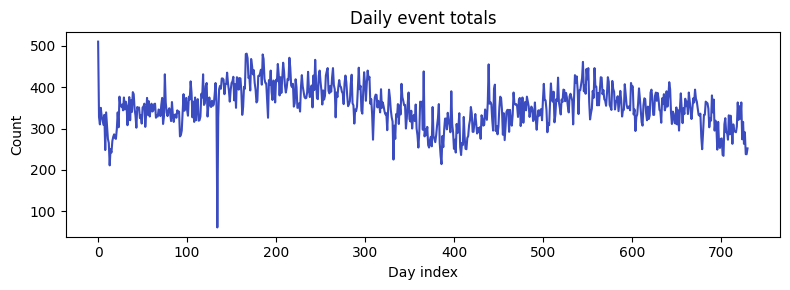
daily_total = counts.sum(axis=0)

plt.figure(figsize=(8, 3))
plt.plot(daily_total, color="#3b4cc0")
plt.title("Daily event totals")
plt.xlabel("Day index")
plt.ylabel("Count")
plt.tight_layout()
plt.show()

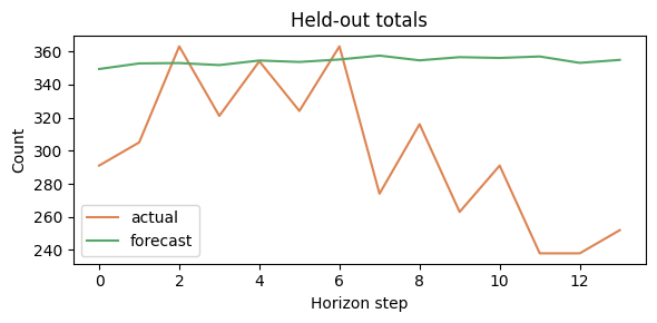
forecast_total = lam.sum(axis=0)
actual_total = y_test.sum(axis=0)

plt.figure(figsize=(6, 3))
plt.plot(actual_total, label="actual", color="#dd8452")
plt.plot(forecast_total, label="forecast", color="#55a868")
plt.title("Held-out totals")
plt.xlabel("Horizon step")
plt.ylabel("Count")
plt.legend()
plt.tight_layout()
plt.show()