Tutorial: Synthetic quickstart (detailed)
This notebook walks through a complete synthetic workflow with full transparency:
Simulate counts on synthetic locations with a travel-time matrix.
Visualize the raw counts and implied mobility.
Grid the space to connect locations to a regular substrate.
Describe the model and its mathematics.
Fit the model and inspect diagnostics.
Reconstruct intensities and compare against data.
Forecast future counts and analyze accuracy.
The goal is to make each step explicit so you can adapt the recipe to real data.
[1]:
## 1. Setup
[ ]:
from __future__ import annotations

import matplotlib.pyplot as plt
import numpy as np
import scipy.sparse as sp

from motac.models import fit_road_hawkes_mle, forecast_intensity_horizon
from motac.models.likelihood import road_intensity_matrix, road_loglik
from motac.sim import discrete_exponential_kernel, simulate_road_hawkes_counts
from motac.spatial.grid_builder import LonLatBounds, build_regular_grid

seed = 0
n_locations = 5
n_steps_train = 40
horizon = 10
n_lags = 6

mu_true = np.full((n_locations,), 0.15, dtype=float)
alpha_true = 0.6
beta_true = 2e-3

rng = np.random.default_rng(seed)
2. Simulate a synthetic world
We create synthetic location coordinates, build a pairwise travel-time matrix, and simulate a discrete-time road-constrained Hawkes process.
y_true: simulated event counts per location and time step.intensity_true: conditional intensity \(\lambda_{i,t}\) implied by the same model.
[3]:
xy = rng.uniform(0.0, 1.0, size=(n_locations, 2))

dx = xy[:, None, 0] - xy[None, :, 0]
dy = xy[:, None, 1] - xy[None, :, 1]
dist = np.sqrt(dx**2 + dy**2)
travel_time_dense = 600.0 * dist
np.fill_diagonal(travel_time_dense, 0.0)
travel_time_s = sp.csr_matrix(travel_time_dense)

mobility = np.exp(-beta_true * travel_time_dense)
kernel_true = discrete_exponential_kernel(n_lags=n_lags, beta=0.8)

y_true = simulate_road_hawkes_counts(
    travel_time_s=travel_time_s,
    mu=mu_true,
    alpha=alpha_true,
    beta=beta_true,
    kernel=kernel_true,
    T=n_steps_train + horizon,
    seed=seed + 1,
)

intensity_true = road_intensity_matrix(
    travel_time_s=travel_time_s,
    mu=mu_true,
    alpha=alpha_true,
    beta=beta_true,
    kernel=kernel_true,
    y=y_true,
)

print("xy shape:", xy.shape)
print("travel_time_s shape:", travel_time_s.shape)
print("y_true shape:", y_true.shape)
print("intensity_true shape:", intensity_true.shape)
world.xy shape: (5, 2)
mobility shape: (5, 5)
y_true shape: (5, 50)
intensity shape: (5, 50)
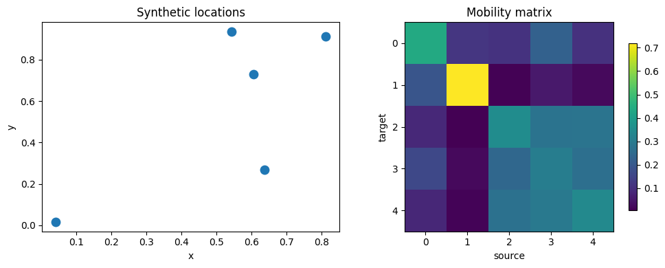
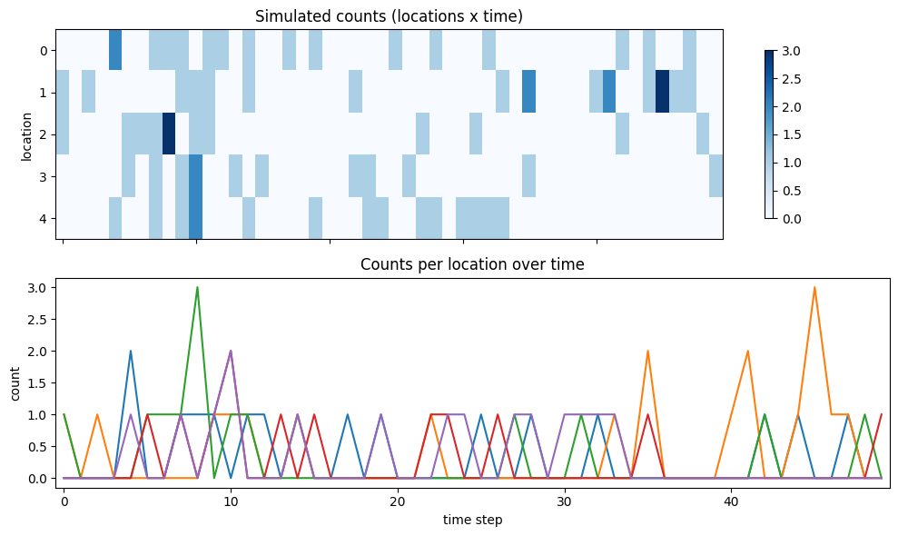
3. Visualize the synthetic data
We’ll inspect the location layout, mobility matrix, and simulated counts over time.
[4]:
fig, axes = plt.subplots(1, 2, figsize=(10, 4))

axes[0].scatter(xy[:, 0], xy[:, 1], s=80, c="tab:blue")
axes[0].set_title("Synthetic locations")
axes[0].set_xlabel("x")
axes[0].set_ylabel("y")

im = axes[1].imshow(mobility, cmap="viridis")
axes[1].set_title("Road kernel matrix W")
axes[1].set_xlabel("source")
axes[1].set_ylabel("target")
fig.colorbar(im, ax=axes[1], shrink=0.8)

plt.tight_layout()
[5]:
fig, axes = plt.subplots(2, 1, figsize=(10, 6), sharex=True)

im0 = axes[0].imshow(y_true, aspect="auto", cmap="Blues")
axes[0].set_title("Simulated counts (locations x time)")
axes[0].set_ylabel("location")
fig.colorbar(im0, ax=axes[0], shrink=0.8)

axes[1].plot(y_true.T)
axes[1].set_title("Counts per location over time")
axes[1].set_xlabel("time step")
axes[1].set_ylabel("count")

plt.tight_layout()
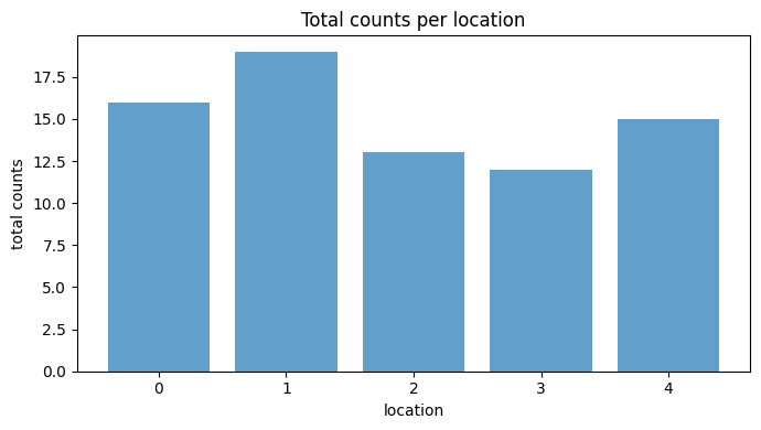
Summary statistics
Before moving to gridding, summarize the counts and intensities per location to see which locations are most active.
[6]:
total_counts = y_true.sum(axis=1)
mean_counts = y_true.mean(axis=1)
mean_intensity = intensity_true.mean(axis=1)

for i in range(n_locations):
    print(
        f"loc {i}: total={total_counts[i]:.0f}, "
        f"mean count={mean_counts[i]:.2f}, "
        f"mean intensity={mean_intensity[i]:.2f}"
    )

fig, ax = plt.subplots(figsize=(7, 4))
ax.bar(np.arange(n_locations), total_counts, color="tab:blue", alpha=0.7)
ax.set_title("Total counts per location")
ax.set_xlabel("location")
ax.set_ylabel("total counts")
plt.tight_layout()
loc 0: total=16, mean count=0.32, mean intensity=0.33
loc 1: total=19, mean count=0.38, mean intensity=0.36
loc 2: total=13, mean count=0.26, mean intensity=0.31
loc 3: total=12, mean count=0.24, mean intensity=0.31
loc 4: total=15, mean count=0.30, mean intensity=0.31
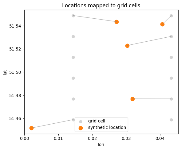
4. Connect locations to a regular grid
Real datasets are often aggregated onto a regular spatial grid. We’ll create a small lon/lat bounding box, build a regular grid, and map each synthetic location to its nearest grid cell. This illustrates how gridding connects raw coordinates to a structured substrate.
[7]:
bounds = LonLatBounds(lon_min=0.0, lon_max=0.05, lat_min=51.45, lat_max=51.55)
grid = build_regular_grid(bounds, cell_size_m=2000.0)

# Map synthetic unit-square coordinates into lon/lat bounds for visualization.
lon = bounds.lon_min + xy[:, 0] * (bounds.lon_max - bounds.lon_min)
lat = bounds.lat_min + xy[:, 1] * (bounds.lat_max - bounds.lat_min)

# Nearest grid cell for each location.
loc_xy = np.column_stack([lon, lat])
grid_xy = np.column_stack([grid.lon, grid.lat])

d2 = ((loc_xy[:, None, :] - grid_xy[None, :, :]) ** 2).sum(axis=2)
nearest_cell = d2.argmin(axis=1)

print("grid cells:", grid.lat.size)
print("nearest cell per location:", nearest_cell)
grid cells: 12
nearest cell per location: [ 3  0 11  9 10]
[8]:
fig, ax = plt.subplots(figsize=(6, 5))
ax.scatter(grid.lon, grid.lat, s=40, c="lightgray", label="grid cell")
ax.scatter(lon, lat, s=80, c="tab:orange", label="synthetic location")

for i, idx in enumerate(nearest_cell):
    ax.plot(
        [lon[i], grid.lon[idx]],
        [lat[i], grid.lat[idx]],
        color="tab:gray",
        linewidth=1,
        alpha=0.6,
    )

ax.set_title("Locations mapped to grid cells")
ax.set_xlabel("lon")
ax.set_ylabel("lat")
ax.legend()
plt.tight_layout()
5. Model definition and math
We fit a discrete-time Hawkes process with spatial coupling:
[ \lambda_i(t) = \mu_i + \alpha `:nbsphinx-math:sum`j W{ij} ; h_j(t) ]
where:
(\mu_i) is the baseline rate for location (i).
is the mobility/influence matrix.
(h_j(t) = \sum{:nbsphinx-math:`ell=1`}^{L} k{\ell} , y_{j,t-\ell}) is a lagged history term.
The kernel (k) is a discrete exponential kernel with decay parameter (\beta).
Counts are modeled as:
[ Y_{i,t} \sim `:nbsphinx-math:text{Poisson}`(\lambda_i(t)). ]
We estimate (\mu), (\alpha), and (\beta) by maximum likelihood using the training window.
6. Fit the Hawkes model
We fit (\mu), (\alpha), and (\beta) by maximum likelihood on the training window.
[9]:
y_train = y_true[:, :n_steps_train]
y_test = y_true[:, n_steps_train: n_steps_train + horizon]

fit = fit_road_hawkes_mle(
    travel_time_s=travel_time_s,
    kernel=kernel_true,
    y=y_train,
    init_alpha=0.2,
    init_beta=1e-3,
    maxiter=200,
)

print("fit keys:", list(fit.keys()))
print("mu_hat:", np.round(fit["mu"], 3))
print("alpha_hat:", round(float(fit["alpha"]), 3))
print("beta_hat:", round(float(fit["beta"]), 6))
print("loglik_init:", round(float(fit["loglik_init"]), 3))
print("loglik_final:", round(float(fit["loglik"]), 3))
fit keys: ['mu', 'alpha', 'beta', 'kernel', 'loglik', 'loglik_init', 'result']
mu_hat: [0.21  0.166 0.113 0.137 0.235]
alpha_hat: 0.426
beta_hat: 0.871
loglik_init: -134.978
loglik_final: -132.59
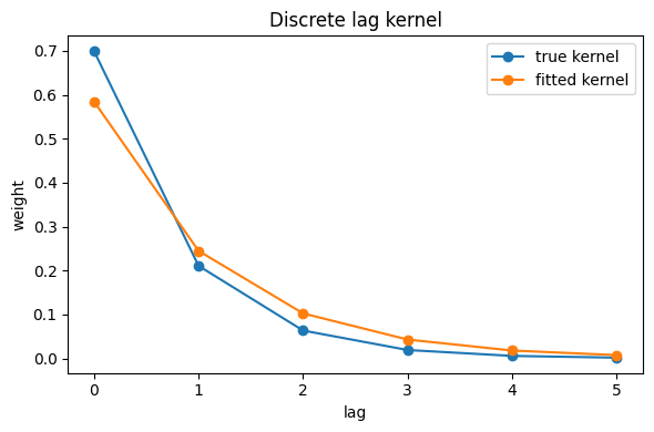
Fit diagnostics
We’ll compare fitted parameters with ground truth. The lag kernel is fixed in this fit, so we also plot the kernel used for simulation and estimation.
[10]:
mu_hat = np.asarray(fit["mu"], dtype=float)
alpha_hat = float(fit["alpha"])
beta_hat = float(fit["beta"])
kernel_hat = np.asarray(kernel_true, dtype=float)

print("mu_true:", np.round(mu_true, 3))
print("mu_hat:", np.round(mu_hat, 3))
print("alpha_true:", alpha_true, "alpha_hat:", round(alpha_hat, 3))
print("beta_true:", beta_true, "beta_hat:", round(beta_hat, 6))

fig, ax = plt.subplots(figsize=(6, 4))
ax.plot(kernel_true, marker="o", label="kernel (true)")
ax.plot(kernel_hat, marker="o", linestyle="--", label="kernel (fit input)")
ax.set_title("Discrete lag kernel")
ax.set_xlabel("lag")
ax.set_ylabel("weight")
ax.legend()
plt.tight_layout()
mu_true: 0.15
mu_hat: [0.21  0.166 0.113 0.137 0.235]
alpha_true: 0.6 alpha_hat: 0.426
beta_true: 1.2 beta_hat: 0.871
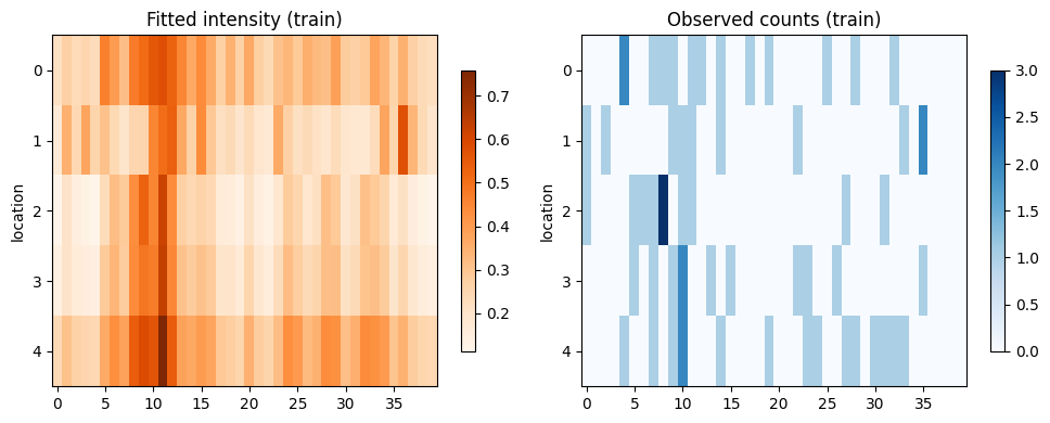
7. Reconstruct intensities on the training window
We reconstruct the conditional intensities (\lambda_{i,t}) under the fitted parameters and compare them to the observed counts. This gives a sanity check on how well the fitted model explains the training data.
[11]:
intensity_hat = road_intensity_matrix(
    travel_time_s=travel_time_s,
    mu=mu_hat,
    alpha=alpha_hat,
    beta=beta_hat,
    kernel=kernel_hat,
    y=y_train,
)

print("intensity_hat shape:", intensity_hat.shape)

fig, axes = plt.subplots(1, 2, figsize=(10, 4))

im1 = axes[0].imshow(intensity_hat, aspect="auto", cmap="Oranges")
axes[0].set_title("Fitted intensity (train)")
axes[0].set_ylabel("location")
fig.colorbar(im1, ax=axes[0], shrink=0.8)

im2 = axes[1].imshow(y_train, aspect="auto", cmap="Blues")
axes[1].set_title("Observed counts (train)")
axes[1].set_ylabel("location")
fig.colorbar(im2, ax=axes[1], shrink=0.8)

plt.tight_layout()
intensity_hat shape: (5, 40)
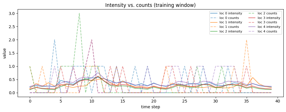
[12]:
fig, ax = plt.subplots(figsize=(10, 4))

for i in range(n_locations):
    ax.plot(intensity_hat[i], color=f"C{i}", alpha=0.7, label=f"loc {i} intensity")
    ax.plot(y_train[i], color=f"C{i}", linestyle="--", alpha=0.5, label=f"loc {i} counts")

ax.set_title("Intensity vs. counts (training window)")
ax.set_xlabel("time step")
ax.set_ylabel("value")
ax.legend(ncol=2, fontsize=8)
plt.tight_layout()
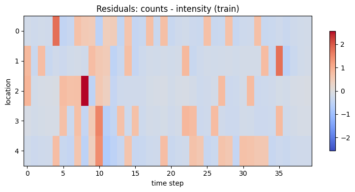
Reconstruction diagnostics
We can quantify how well the fitted model explains the training data using the Poisson log-likelihood and a simple error heatmap.
[13]:
train_loglik = road_loglik(
    travel_time_s=travel_time_s,
    mu=mu_hat,
    alpha=alpha_hat,
    beta=beta_hat,
    kernel=kernel_hat,
    y=y_train,
    family="poisson",
)

# Poisson log-likelihood per event/time step for interpretability.
ll_per_step = train_loglik / max(n_locations * n_steps_train, 1)

residual = y_train - intensity_hat

print(f"Train log-likelihood: {train_loglik:.2f}")
print(f"Log-likelihood per step: {ll_per_step:.4f}")

fig, ax = plt.subplots(figsize=(8, 4))

im = ax.imshow(
    residual,
    aspect="auto",
    cmap="coolwarm",
    vmin=-np.max(np.abs(residual)),
    vmax=np.max(np.abs(residual)),
)
ax.set_title("Residuals: counts - intensity (train)")
ax.set_ylabel("location")
ax.set_xlabel("time step")
fig.colorbar(im, ax=ax, shrink=0.8)

plt.tight_layout()
Train log-likelihood: -132.59
Log-likelihood per step: -0.6629
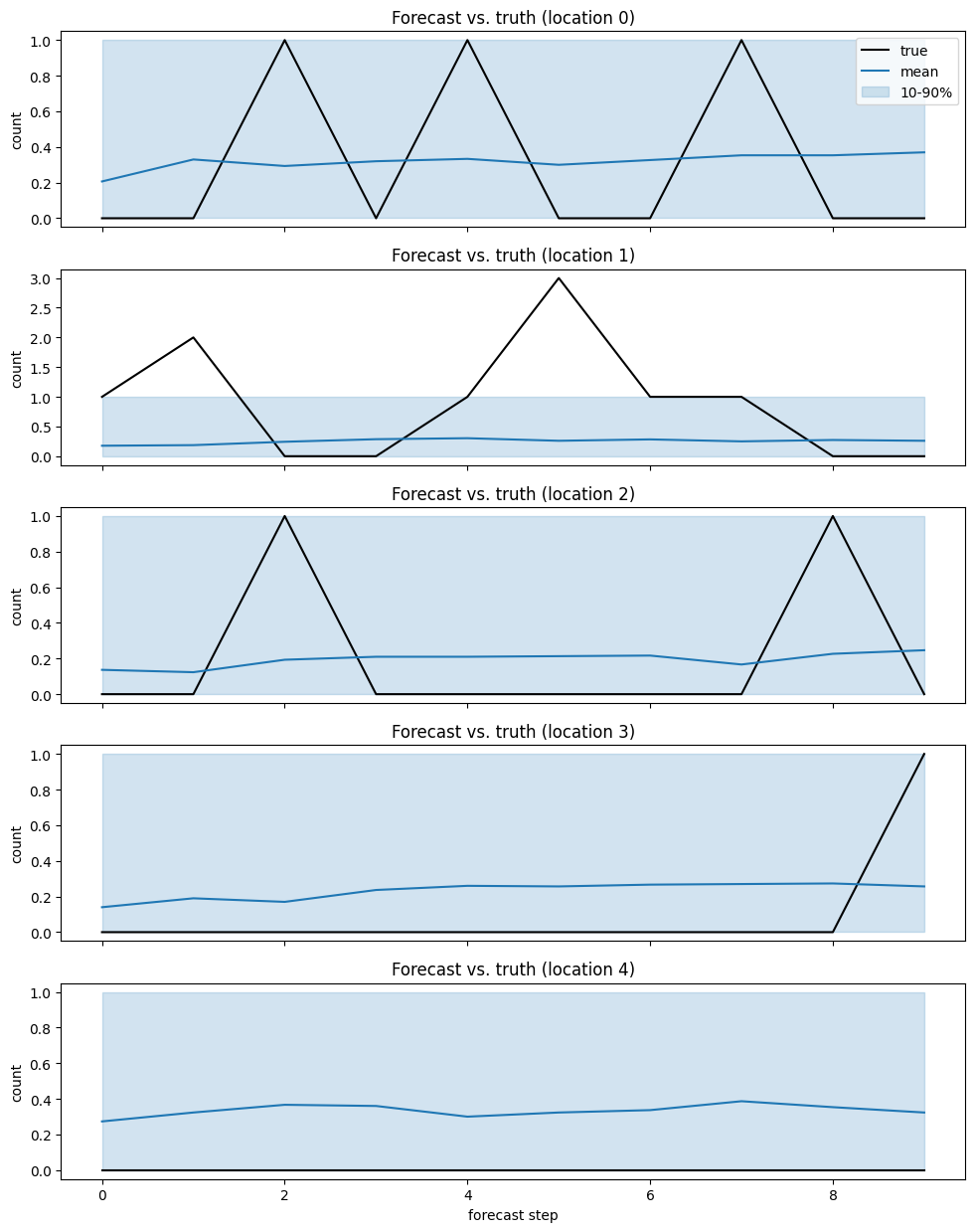
8. Forecast the future and evaluate accuracy
We forecast the next horizon steps deterministically, then sample Poisson paths around those mean intensities to build predictive intervals.
[14]:
n_paths = 300

lam_forecast = forecast_intensity_horizon(
    travel_time_s=travel_time_s,
    mu=mu_hat,
    alpha=alpha_hat,
    beta=beta_hat,
    kernel=kernel_hat,
    y_history=y_train,
    horizon=horizon,
)

# Keep sampling numerically stable for tutorial execution.
lam_safe = np.nan_to_num(lam_forecast, nan=0.0, posinf=1e6, neginf=0.0)
lam_safe = np.clip(lam_safe, 0.0, 1e6)

rng_paths = np.random.default_rng(seed + 2)
y_paths = rng_paths.poisson(
    lam=lam_safe[None, :, :],
    size=(n_paths,) + lam_forecast.shape,
).astype(float)

y_mean = y_paths.mean(axis=0)
y_q = np.quantile(y_paths, [0.1, 0.5, 0.9], axis=0)

print("lam_forecast shape:", lam_forecast.shape)
print("lam_safe max:", float(lam_safe.max()))
print("y_paths shape:", y_paths.shape)
print("y_mean shape:", y_mean.shape)
print("y_q shape:", y_q.shape)
y_paths shape: (300, 5, 10)
y_mean shape: (5, 10)
y_q shape: (3, 5, 10)
[15]:
fig, axes = plt.subplots(n_locations, 1, figsize=(10, 2.5 * n_locations), sharex=True)

for i, ax in enumerate(axes):
    ax.plot(y_test[i], color="black", label="true")
    ax.plot(y_mean[i], color="tab:blue", label="mean")
    ax.fill_between(
        np.arange(horizon),
        y_q[0, i],
        y_q[2, i],
        color="tab:blue",
        alpha=0.2,
        label="10-90%",
    )
    ax.set_title(f"Forecast vs. truth (location {i})")
    ax.set_ylabel("count")

axes[-1].set_xlabel("forecast step")
axes[0].legend(loc="upper right")
plt.tight_layout()
[16]:
rmse = float(np.sqrt(np.mean((y_test - y_mean) ** 2)))
mae = float(np.mean(np.abs(y_test - y_mean)))

coverage = float(np.mean((y_test >= y_q[0]) & (y_test <= y_q[2])))

print(f"RMSE: {rmse:.3f}")
print(f"MAE: {mae:.3f}")
print(f"80% interval coverage: {coverage:.3f}")
RMSE: 0.618
MAE: 0.442
80% interval coverage: 0.960